Domains & meshes — Scimba Jax

1 · No mesh

Mesh-less domains

Sampled on the fly, at every training step: a domain is a level set plus a mapping, and a solver only ever sees the points a sampler drew from it.

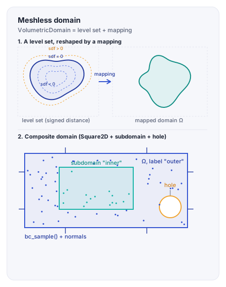
A level set (signed distance contours) reshaped by a mapping into a curved domain, and below it a composite meshless domain made of an outer square, an inner subdomain and a hole, sampled by random interior and boundary points with normals.

Every VolumetricDomain is defined by a level set (a signed distance function, tested as sdf(x) < 0) and reshaped by a mapping; below, a main domain built that way also carries a subdomain and a hole, sampled by a DomainSampler (interior points, boundary points and normals).

1. A volumetric domain, with a subdomain and a hole

A VolumetricDomain that is a main domain can be extended with subdomains, holes and a mapping. Each piece carries its own label, which shows up as a key in the dictionaries returned by samplers.

Square2D and Disk2D come from domains/meshless_domains/; arbitrary-dimension equivalents (HypercubeND, BallND) live in domains_nd.py. Under the hood, each is just a level set and a mapping — see below.

from scimba_jax.domains.meshless_domains.domains_2d import Square2D, Disk2D

bounds_outer = [(-1.0, 1.0), (-1.0, 1.0)]
bounds_inner = [(-0.7, 0.3), (-0.25, 0.25)]

outer = Square2D(bounds_outer, is_main_domain=True, label_str="outer")
inner = Square2D(bounds_inner, is_main_domain=False, label_str="inner")
hole = Disk2D((0.55, 0.0), 0.2, is_main_domain=False, label_str="hole")

outer.add_subdomain(inner)
outer.add_hole(hole)

2. Defining a domain from a level set and a mapping

A VolumetricDomain is fundamentally a SignedDistance (the level set: < 0 inside, > 0 outside) plus bounds. Square2D, Disk2D and friends are thin wrappers around this pattern; you can write the same thing directly, then reshape it with a Mapping.

import jax.numpy as jnp
from scimba_jax.domains.sdf import SignedDistance
from scimba_jax.domains.meshless_domains.base import VolumetricDomain
from scimba_jax.domains.domain_mapping import DomainMapping as Mapping


class Disk2DSignedDistance(SignedDistance):
    def __init__(self, center, radius):
        super().__init__(dim=2, threshold=0.0)
        self.center = center
        self.radius = radius

    def _sdf_pointwise(self, x):
        return (jnp.linalg.norm(x - self.center, axis=0) - self.radius)[None]


disk = VolumetricDomain(
    domain_type="Disk2D",
    dim=2,
    sdf=Disk2DSignedDistance(jnp.array([0.0, 0.0]), 1.0),
    bounds=[(-1.0, 1.0), (-1.0, 1.0)],
    is_main_domain=True,
)

disk.set_mapping(
    Mapping.rot_2d(angle=jnp.pi / 6.0, center=jnp.array([0.0, 0.0])),
    [(-1.5, 1.5), (-1.5, 1.5)],
)

3. Mapping propagates to subdomains and holes

Calling set_mapping on a composite main domain — like outer from step 1 — reshapes it and automatically propagates the same mapping to its subdomains and holes. Built-ins cover common cases such as rotations; custom mappings are plain JAX-traceable functions, so vmap and autodiff (e.g. for normals) work out of the box.

import jax.numpy as jnp
from scimba_jax.domains.domain_mapping import DomainMapping as Mapping

outer.set_mapping(
    Mapping.rot_2d(angle=jnp.pi / 3.0, center=jnp.array([0.0, 0.0])),
    [(-2.0, 2.0), (-2.0, 2.0)],
)

4. Boundary domains are parameterized curves

A boundary piece is a SurfacicDomain: a 1D parametric_domain (an interval) mapped into physical space by a surface (a DomainMapping). Segment2D, Circle2D and ArcCircle2D are built exactly this way — ArcCircle2D simply maps an angle interval through Mapping.circle.

Splitting hole's boundary into two named arcs and registering them with add_bc_domain lets you target each one independently — e.g. with different boundary conditions north vs. south.

import jax.numpy as jnp
from scimba_jax.domains.meshless_domains.domains_2d import ArcCircle2D

# split the hole's circular boundary into two named, parameterized arcs
disk_up = ArcCircle2D((0.55, 0.0), 0.2, (0.0, jnp.pi), label_str="bc hole north")
disk_down = ArcCircle2D(
    (0.55, 0.0), 0.2, (jnp.pi, 2 * jnp.pi), label_str="bc hole south"
)

hole.add_bc_domain(disk_up)
hole.add_bc_domain(disk_down)

A parametric angle interval [0, 2π], split into [0, π] and [π, 2π], mapped via Mapping.circle onto a physical circle whose top half is the 'bc hole north' arc and bottom half is the 'bc hole south' arc, with arrows showing the parameterization direction.

A boundary curve is just a parametric domain (here an angle interval) pushed through a surface mapping. Splitting [0, 2π] into [0, π] and [π, 2π] and mapping each half with Mapping.circle gives two independent boundary pieces — the same construction used by ArcCircle2D above, and how the north/south boundary conditions on hole are told apart.

2 · Built once

Meshes

Four kinds, chosen by geometry rather than by solver: a single mapped grid, an arbitrary boundary imported through Gmsh, a handful of smooth patches, or the product of two meshes already in hand.

1. A structured mesh for the DG/FEM solver

Classical solvers (linear_approximation/dg/) work on a Mesh instead: a cartesian grid of n_cells reference cells, each with its own Gauss quadrature (ref_quad), mapped to physical space through the same Mapping abstraction as the mesh-less domains above.

Adapted from the diffusion–advection DG example — view source ↗.

from scimba_jax.linear_approximation.meshes.mesh import Mesh
from scimba_jax.linear_approximation.quad.gauss_quad import UnitSquareTensorized
from scimba_jax.mapping.mapping import InvertibleFunction, Mapping

physical_dim = 2
quad_order = 3
n_cells = 40

mapping_id = InvertibleFunction(lambda x: x, lambda y: y)

mesh = Mesh(
    dim=physical_dim,
    n_cells=(n_cells, n_cells),
    ref_quad=UnitSquareTensorized(dim=physical_dim, order=quad_order),
    mapping=Mapping(mappings=[mapping_id]),
)

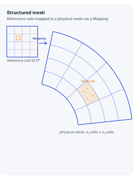
A structured reference cell mapped through a Mapping object onto a curved physical mesh, with Gauss quadrature points.

One reference cell, [0, 1]², mapped onto a physical Mesh by the same Mapping abstraction — here onto a curved sector; every cell carries its own Gauss quadrature points.

2. Unstructured quads, imported through Gmsh

Use an unstructured mesh when a curved or arbitrary boundary is not naturally described by one mapping. Gmsh returns a MacroMesh with complete tensor-product quadrilaterals; UnstructuredMesh.from_macro_mesh turns it into the mesh consumed by a solver.

Gmsh is optional: install scimba[mesh]. The requested geometry order is retained, including the nodes on curved cell edges.

import numpy as np
from scimba_jax.linear_approximation.meshes.unstructured_mesh import UnstructuredMesh
from scimba_jax.linear_approximation.quad.gauss_quad import UnitSquareTensorized
from scimba_jax.mapping.macro_mesh import macro_mesh_from_points

# Requires: pip install scimba[mesh]
# Gmsh closes this ordered boundary and fills it with curved Q_p cells.
boundary = np.array([[-1.0, -0.7], [0.8, -0.9], [1.2, 0.1], [0.2, 1.0], [-0.9, 0.6]])
macro = macro_mesh_from_points(boundary, order=3, mesh_size=0.18, smooth=True)

mesh = UnstructuredMesh.from_macro_mesh(
    macro,
    UnitSquareTensorized(dim=2, order=5),
)

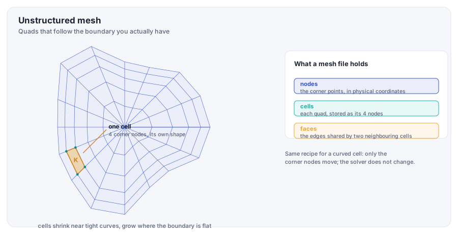
A mesh of quadrilateral cells following a smooth curved boundary, with one cell K highlighted and its four corner nodes marked, and a box listing what a mesh file holds: nodes (physical coordinates), cells (each quad's 4 nodes) and faces (the edges shared by two neighbouring cells).

A mesh is just points (nodes), the quads they form (cells), and which quads touch (faces). Cells shrink near a tight curve and grow where the boundary is flat; a curved cell follows the same recipe — only its corner nodes move.

3. Block-structured meshes for patchwise geometry

This representation is useful when a domain has a small number of smooth patches — for example an O-grid around a disk or hole. Every patch has its own mapped Cartesian grid, while the container owns the interface pairings. Patches may use different resolutions when an interface is non-conforming.

For DG, an interface uses the same numerical flux as an interior face. For continuous FEM, supply an explicit Nitsche/SIPG interface flux: there is deliberately no implicit penalty choice.

from scimba_jax.linear_approximation.meshes.block_structured_mesh import BlockStructuredMesh
from scimba_jax.linear_approximation.quad.gauss_quad import UnitSquareTensorized
from scimba_jax.mapping.macro_mesh import macro_mesh_ogrid_disk

# Five macro-patches: a square centre plus four curved outer patches.
macro = macro_mesh_ogrid_disk(radius=1.0, inner=0.45, n=1, order=3)
quad = UnitSquareTensorized(dim=2, order=5)

# One structured 12 x 12 mesh in every patch.
mesh = BlockStructuredMesh(macro, n_cells=(12, 12), ref_quad=quad)

# Per-patch counts are also valid, e.g. [(8, 8), (16, 16), ...].

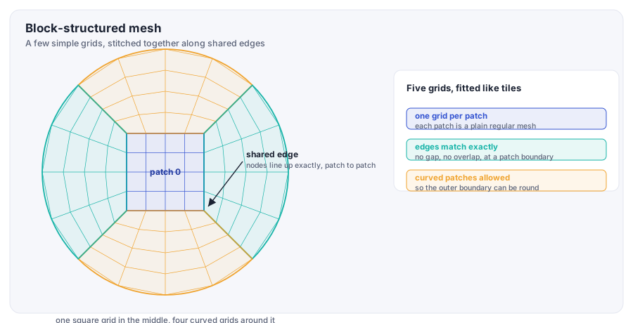
Five patches around a curved boundary: a square grid in the middle and four curved grids around it, meeting exactly at their shared edges, with a box listing three properties: one grid per patch, edges match exactly, and curved patches are allowed.

Each patch is an ordinary regular grid; five of them, sharing edges exactly, make one mesh whose outer boundary can be round even though every single patch is simple.

4. Tensor meshes: the product of two meshes already in hand

tensor_mesh(mesh_a, mesh_b) builds no new mesh class: a cell of the product is cell_a × cell_b, its quadrature is quad_a ⊗ quad_b, and the result is an ordinary Mesh, BlockStructuredMesh or UnstructuredMesh — whichever of the two factors is the least structured. Everything already written for that class keeps working unchanged: faces, fluxes, the fast Cartesian paths.

This is how a space-time slab, a phase-space mesh, or a toroidal tokamak cross-section gets built: as the product of two ordinary meshes, with names so the physics reads f(x, t) rather than slices of a flat array, and periodic_directions to glue an axis of the product — the toroidal angle, say.

from scimba_jax.linear_approximation.meshes.mesh import Mesh
from scimba_jax.linear_approximation.meshes.tensor_mesh import tensor_mesh
from scimba_jax.linear_approximation.quad.gauss_quad import UnitSquareTensorized
from scimba_jax.mapping.mapping import InvertibleFunction, Mapping


def _line(n_cells, length, order=3):
    physical = InvertibleFunction(lambda x: length * x, lambda y: y / length)
    return Mesh(
        dim=1,
        n_cells=(n_cells,),
        ref_quad=UnitSquareTensorized(dim=1, order=order),
        mapping=Mapping(mappings=[physical]),
    )


# A 1-D mesh in x, times a 1-D mesh in t: one 2-D space-time slab, no
# time-stepping. The product is a plain `Mesh` -- the LEAST structured of
# its two factors -- so every DG/FEM scheme works on it unchanged.
mesh_x, mesh_t = _line(32, length=1.0), _line(12, length=0.1)
slab = tensor_mesh(mesh_x, mesh_t, names=("x", "t"))

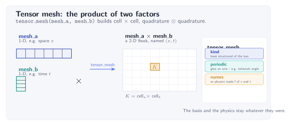
mesh_a, a 1-D structured mesh in x, and mesh_b, a 1-D structured mesh in t, combined by tensor_mesh into mesh_a times mesh_b: a 2-D Mesh named (x, t), with one cell K equal to cell_a times cell_b highlighted. A box lists three properties: kind (least structured of the two), periodic (glue an axis, e.g. tokamak angle) and names (so physics reads f of x and t).

Two 1-D meshes in, one 2-D mesh out: the product is a plain Mesh because both factors already were. The basis and the physics stay whatever they were on either factor — the tensor structure lives in the mesh and its connectivity, not in the basis.

For the full walkthrough — holes, custom boundaries, kinetic/parametric domains, generic N-dimensional domains — see the Domains and samplers tutorial, or the Scimba Jax API reference.