Samplers — Scimba Jax

Top: a bounding box with uniformly scattered points, some teal (accepted, inside the level set) and some gray (rejected, outside), mapped onto a final teal point cloud labelled dict with key outer mapping to a one-tuple of points. Bottom: a parametric interval mapped through a surface plus normals onto a boundary arc with normal ticks, labelled dict with key boundary mapping to a tuple of points and normals.

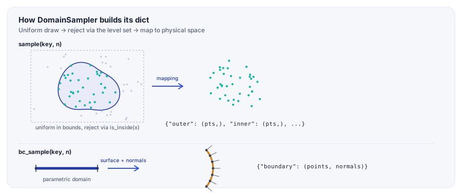
Top — VolumetricSampler draws points uniformly in the domain's bounding box, keeps only those with is_inside(x) (the level set test), and pushes survivors through the domain's mapping. Bottom — SurfacicSampler samples the boundary's parametric domain directly (no rejection needed there) and pushes points through the surface mapping, computing normals from its Jacobian.

1. Rejection sampling against the level set

VolumetricSampler is the building block: it estimates what fraction of the bounding box the domain occupies (a quick Monte-Carlo calibration pass), then loops — draw a batch uniformly in domain.bounds, keep the ones with is_inside(x) (the sdf test from the level set, also excluding holes), repeat until enough points survive — before mapping them to physical space.

import jax
from scimba_jax.nonlinear_approximation.integration.monte_carlo import (
    VolumetricSampler,
)

# VolumetricSampler.sample(key, n) does, internally:
#   1. draw points uniformly in domain.bounds        (BoxSampler)
#   2. keep only points where domain.is_inside(x)     (the level set test)
#   3. repeat until n points have been accepted
#   4. push the accepted points through domain.mapping (if the domain is mapped)
vsampler = VolumetricSampler(outer)
key, pts = vsampler.sample(jax.random.PRNGKey(0), 2000)

2. Sampling the interior: sample()

DomainSampler wraps one VolumetricSampler per labelled piece: the main domain minus its subdomains and holes, plus each subdomain (also minus holes). Holes have no interior sampler — they're cut out, never sampled.

Each dict key is exactly the piece's get_label() — the label_str given when the domain was built (plus a numeric suffix if label_idx != 0); a domain built without an explicit label defaults to "interior". In practice you rarely call DomainSampler.sample() on its own — see §3.

from scimba_jax.nonlinear_approximation.integration.monte_carlo import DomainSampler

sampler = DomainSampler(outer)
key, samples = sampler.sample(jax.random.PRNGKey(0), 2000)

list(samples.keys())
# ['outer', 'inner']
# one label per "in" piece: the main domain (minus its subdomains/holes)
# and each subdomain. Holes have no interior sampler -- they're cut out.

samples["outer"]
# (Array of shape (n_outer, 2),)   <- always a 1-tuple

3. What you actually call: TensorizedSampler

Real training code doesn't call bc_sample() directly. It wraps the DomainSampler (and any other axis — time, parameters...) in a TensorizedSampler(..., bc=True) and makes one sample(key, n, n_bc) call, which merges interior and boundary points into a single flat dict — that's the dict a Projector/loss function actually consumes.

By default every boundary piece belongs to one group, "boundary" (domain.boundaries = {"boundary": [""]}). Split it with set_boundaries_dict(...) to get one key per edge (or per boundary condition) — e.g. a Dirichlet/Neumann square below groups its four edges into "bc N" and "bc D", and those keys drive both the residual and the loss weights directly.

from scimba_jax.nonlinear_approximation.integration.monte_carlo import (
    DomainSampler,
    TensorizedSampler,
)

sampler = TensorizedSampler([DomainSampler(outer)], bc=True)

# one call samples interior AND boundary, merged into a single dict
key, sample_dict = sampler.sample(jax.random.PRNGKey(0), 2000, 2000)

list(sample_dict.keys())
# ['outer', 'inner', 'boundary']
# "outer" / "inner" come from DomainSampler.sample()    -> (points,)
# "boundary"        comes from DomainSampler.bc_sample() -> (points, normals)

4. Boundary groups, by example

One group per condition, not per edge name: "bc N" covers the north edge (Neumann), "bc D" covers the other three (Dirichlet) — Square2D's default boundary labels ("bc north", "bc south", ...) are just substrings to match against.

Adapted from view source ↗.

from scimba_jax.domains.meshless_domains.domains_2d import Square2D
from scimba_jax.nonlinear_approximation.integration.monte_carlo import (
    DomainSampler,
    TensorizedSampler,
)

domain_x = Square2D([[0.0, 1.0], [0.0, 1.0]], is_main_domain=True)
domain_x.set_boundaries_dict(
    {
        "bc N": ["bc north"],  # Neumann on the north edge
        "bc D": ["bc east", "bc south", "bc west"],  # Dirichlet elsewhere
    }
)

sampler = TensorizedSampler([DomainSampler(domain_x)], bc=True)
key, sample_dict = sampler.sample(key, N_COLLOC, N_BC_COLLOC)
# sample_dict.keys() -> ['interior', 'bc N', 'bc D']

weights = {"interior": [1.0], "bc N": [30.0], "bc D": [30.0]}

5. The shape of what comes back

DomainSampler.sample() and .bc_sample() each return (key, dict) with the same convention — domain/group label → tuple — but a different tuple width; TensorizedSampler merges both into the one flat dict your loss function actually sees (Projector looks up each residual by exactly these keys). Stacking more axes (time, parameters...) extends every per-label tuple in place, ordered by model_type, and prefixes initial-condition entries with "ic ".

SAMPLE_TYPE = dict[str, tuple[jnp.ndarray, ...]]

# DomainSampler.sample(key, n)     -> {label:       (points,)}
# DomainSampler.bc_sample(key, n)  -> {group_label: (points, normals)}
#
# TensorizedSampler([DomainSampler(domain)], bc=True).sample(key, n, n_bc)
# merges both -- this is the dict a Projector actually consumes:
# {label: (points,), ..., group_label: (points, normals), ...}

6. Writing a new sampler

Not for the spatial ("x") slot — that one is special-cased: TensorizedSampler requires it to be a real DomainSampler (isinstance check), and DomainSampler is everything covered in §1–4: rejection sampling, subdomain/hole bookkeeping, boundary grouping. You don't rewrite that machinery for a new shape — you implement a new domain (a level set + mapping, see Domains & meshes) and the existing DomainSampler wraps it for free.

For every other axis (time, parameters, velocity, anything custom), it really is that simple — the "sampler" interface there is duck-typed, no base class: just sample(key, n) -> (key, array) and a JIT-friendly build_sample_func(n) -> Callable. UniformTimeSampler is the whole pattern — wrap a BoxSampler, no rejection needed since these domains are plain intervals/boxes. The only other special case: the time ("t") slot must specifically be a UniformTimeSampler.

from scimba_jax.nonlinear_approximation.integration.monte_carlo_box import (
    BoxSampler,
)


class UniformTimeSampler:
    def __init__(self, bounds: tuple[float, float]):
        self.bounds = bounds
        self.base_sampler = BoxSampler([self.bounds])

    def sample(self, key, n):
        return self.base_sampler.sample(key, n)

    def build_sample_func(self, n):
        return self.base_sampler.build_sample_func(n)

For samplers over time, parameters, velocity and tensorized combinations, see the Domains and samplers tutorial, or the Scimba Jax API reference.