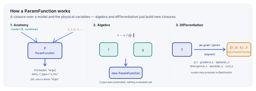
A ParamFunction wraps fn(model, *physical_args):
model is the nonlinear part (a network's own parameters,
θ) and, in the DG/FEM setting, there is also a linear part —
local basis DOFs, called "dofsl" in the code. Algebra and
differentiation never evaluate eagerly: every operator returns a new
ParamFunction, vmapped over collocation points only later.
1. ParamFunction: a closure, not a value
A PDE unknown is represented as \(u(x;\theta)\) for a PINN, or
\(u(x;\theta,\alpha)\) in the DG/FEM setting, where α are the
local linear degrees of freedom of a basis expansion. Both live behind
the same interface: a ParamFunction(dims, fn, f_type)
wrapping fn(model, *args) — model first,
then the physical variables named by f_type (e.g.
"x_mu").
.freeze("model") stops the gradient through θ
(the nonlinear part); .freeze("dofsl") stops it through
α instead (DG variables only) — the nonlinear/linear split
the math suggests, expressed as two gradient targets on one object.
from scimba_jax.nonlinear_approximation.model_class.funcparam_vectorial import (
    ParamScalarFunction,
)

# u(x; theta) = model(x); theta = the network's own (nonlinear) parameters
u = ParamScalarFunction({"x": 2}, fn=lambda model, x: model(x), f_type="x")

u_frozen = u.freeze()         # stop gradient w.r.t. theta (the model)
u_frozen = u.freeze("dofsl")  # DG only: stop gradient w.r.t. the linear DOFs
2. Algebra
Binary operators promote f_type to the union of both
operands' variables (e.g. f(x,μ) * g(t,x,μ) → h(t,x,μ))
and return a new, unevaluated ParamFunction. Overloaded:
+ − * / (elementwise), << (composition,
f << g means f∘g), and @
(matrix/vector product, on ParamFieldFunction /
ParamMatrixFunction).
# elementwise algebra builds a new ParamFunction -- nothing is evaluated yet
residual = u - u_exact          # __sub__
scaled = 2.0 * u                # __rmul__
ratio = u / v                   # __truediv__

# composition: h(*args) = f(g(*args))
h = f << g                      # __lshift__

# matrix-vector product (ParamFieldFunction / ParamMatrixFunction only)
diffusion_flux = A @ grad_u     # __matmul__
3. Differentiation
Every differential operator applies jax.grad /
jacrev / jacfwd / hessian to the
ParamFunction's own __call__, with
argnums resolved from f_type (so
.gradient_x() differentiates w.r.t. whichever argument is
named "x"). The result is wrapped back into a
ParamFunction — often a different subtype, e.g. a scalar's
gradient is a field.
grad_u = u.gradient_x()   # jax.grad(u, argnums=argnums["x"])  -> ParamFieldFunction
lap_u = u.laplacian_x()   # trace(hessian(u, x))                -> ParamScalarFunction
div_q = q.divergence_x()  # trace(jacobian(q, x))               -> ParamScalarFunction
dt_u = u.d_t()             # jax.jacrev(u, argnums=argnums["t"])  -> ParamScalarFunction
J = u.jacobian_x()         # full Jacobian                        -> ParamFieldFunction
4. The family
ParamFunction is the base class.
ParamVecFunction extends it for fixed-size vector output;
ParamFieldFunction and ParamScalarFunction extend
that (a field's size is the spatial dimension, a scalar's is
always 1). ParamMatrixFunction is a separate sibling, directly
under ParamFunction, for matrix-valued output (e.g. a
Jacobian).
u = ParamScalarFunction({"x": 2}, fn=lambda model, x: model(x), f_type="x")
n = ParamFieldFunction({"x": 2}, fn=lambda *a: normal(a[1]), f_type="x", main_var="x")
w = ParamVecFunction(3, {"x": 2}, fn=lambda model, x: model(x), f_type="x")

# the model's own Jacobian -- built by evaluators.py, not by hand
J = ParamMatrixFunction(func.dims, jacrev_theta, func.f_type)
ParamScalarFunction
gradient_x() / laplacian_x()
\(\nabla u\) and \(\Delta u\) — a field and a scalar, respectively.
anisotropic_laplacian_x(A)
\(-\nabla\cdot(A\nabla u)\) for a matrix-valued A.
advection_x(v) / bracket_x(g)
\(v\cdot\nabla u\), and the Poisson bracket \((\nabla u\times\nabla g)\cdot e\).
hessian_x() / det_hessian_x()
Full Hessian, and its (log-)determinant (Monge–Ampère).
ParamFieldFunction
dot(other)
Dot product with another field → a ParamScalarFunction.
divergence_x() / curl_x()
\(\nabla\cdot F\), and \(\nabla\times F\) (scalar in 2D, vector in 3D).
jacobian_x()
\(\partial F/\partial x\) → a ParamMatrixFunction.
laplacian_x()
Vector Laplacian, component-wise trace of the Hessian.
ParamVecFunction
component(i) / components()
Extract one (or all) scalar component(s).
cat(funcs)
Classmethod: concatenate several Param*Functions into one.
@ (__matmul__)
Matrix/vector product with a field or matrix.
ParamMatrixFunction
det() / abs_det()
(Absolute) determinant → a ParamScalarFunction.
not vector-like
No .component()/.cat() — a sibling of
ParamVecFunction, not a subclass.
5. Residual: the strong-form abstraction
A Residual doesn't compute a number — its
construct_residual(*rho) takes the model's
ParamFunction output(s) and returns another
ParamFunction: the pointwise residual, evaluated later at
every sampled point. DirichletResidual is the identity
(compared against g(x) downstream);
NeumannResidual dots the gradient with the boundary
normal — itself just another ParamFieldFunction pulled
out of the sampled "n" argument.
class AbstractResidual(ScimbaPytree):
    @abstractmethod
    def construct_residual(
        self, *rho: PARAM_FUNC_TYPE, precomputed: dict | None = None
    ) -> PARAM_FUNC_TYPE:
        """Build the residual from the model's outputs.

        Evaluated later, vmapped over sampled collocation points.
        """


class DirichletResidual(BoundaryResidual):
    def construct_residual(self, *vars):
        rho = vars[0]
        return rho  # compared against f_rhs = g(x) downstream


class NeumannResidual(BoundaryResidual):
    def construct_residual(self, *vars):
        rho = vars[0]
        grad_x_rho = rho.gradient_x()
        n_model = ParamFieldFunction(
            rho.dims, lambda *args: args[rho.argnums["n"]], rho.f_type
        )
        return grad_x_rho.dot(n_model)  # d(u)/dn
6. AbstractPhysicalModel: wiring residuals to labels
A model's physical_residuals dict maps exactly the labels
the sampler produces ("interior", "bc N",
"bc D"... — see Samplers, §4)
to a Residual. Projector iterates this dict,
looks up each label in the sample dict, and squares/weights every
residual into its own loss term (boundary/initial residuals default to
weight 10 vs. 1 for the interior).
class Projection(AbstractPhysicalModel):
    def __init__(self, main_domain, size, model_type, f_rhs):
        super().__init__(main_domain=main_domain)
        self.physical_residuals = {
            "interior": IdResidual(
                domain=main_domain, size=1, model_type="x_mu", f_rhs=f_rhs
            ),
        }
        # add "bc N", "bc D", ... here too -- same labels the sampler
        # produces (see Samplers, §4); Projector looks each one up by key.
7. AbstractLinearWeakForm: bilinear_form + linear_form
For the classical DG/FEM solver, the model is genuinely weak-form: a
bilinear form \(a(u,v)\) and a linear form \(l(v)\), functions
of both a trial and a test ParamFunction,
assembled into a linear system — not a pointwise residual squared into
a PINN loss. get_fields() auto-wraps each coefficient
attribute (matrices, vectors, scalars) into the right Param*Function
subtype.
class AbstractLinearWeakForm(ScimbaPytree):
    def __init__(self, dim: int): ...

    @abstractmethod
    def bilinear_form(
        self, u: list[PARAM_FUNC_TYPE], v: list[PARAM_FUNC_TYPE]
    ) -> PARAM_FUNC_TYPE:
        """Compute the bilinear form a(u, v)."""

    @abstractmethod
    def linear_form(self, v: list[PARAM_FUNC_TYPE]) -> PARAM_FUNC_TYPE:
        """Compute the linear form l(v)."""
8. Residual-style models, worked
Five real InteriorResidual subclasses from
physical_models/ — same pattern every time: pull the
ParamFunction(s) out of *vars, combine them with
algebra and differentiation, return the residual.
LaplacianResidual
\(-\Delta u = f\)
class LaplacianResidual(InteriorResidual):
    def __init__(self, domain, f_rhs=None, model_type="x"):
        super().__init__(
            domain=domain, size=1, model_type=model_type, f_rhs=f_rhs
        )

    def construct_residual(self, *vars):
        rho = vars[0]
        return -rho.laplacian_x()
GeneralEllipticResidual
\(-\nabla\cdot(A\nabla u) + \mathbf{b}\cdot\nabla u + cu = f\)
class GeneralEllipticResidual(InteriorResidual):
    def __init__(self, domain, model_type="x", f_rhs=None, A=None, b=None, c=None):
        super().__init__(
            domain=domain, size=1, model_type=model_type, f_rhs=f_rhs
        )
        self.A, self.b, self.c = A, b, c

    def construct_residual(self, *vars):
        rho = vars[0]
        result = rho.anisotropic_laplacian_x(self.A)
        if self.b is not None:
            result = result + rho.advection_x(self.b)
        if self.c is not None:
            result = result + rho * self.c
        return result
This is also the time-independent anisotropic diffusion
residual: A is any matrix field, not just the identity —
drop b/c for pure diffusion.
NavierStokesResidual
\((\mathbf{u}\cdot\nabla)\mathbf{u} - \nu\Delta\mathbf{u} + \nabla p = \mathbf{f},\quad \nabla\cdot\mathbf{u} = 0\)
class NavierStokesResidual(InteriorResidual):
    def __init__(self, domain, dim=2, nu=1.0, mode="vec", f_rhs=None, model_type="x"):
        super().__init__(
            domain=domain, size=dim + 1, model_type=model_type, f_rhs=f_rhs
        )
        self.nu, self.dim, self.mode = nu, dim, mode

    def construct_residual(self, *vars):
        u, p = _extract_u_p(vars, self.mode, self.dim)
        lap_u = u.laplacian_x()
        momentum = [
            u.component(i).advection_x(u) - self.nu * lap_u.component(i)
            + p.partial_derivative_x(i)
            for i in range(self.dim)
        ]
        return ParamVecFunction.cat(momentum + [u.divergence_x()])
WaveResidual
\(\partial_{tt} u - \Delta u = f\)
class WaveResidual(InteriorResidual):
    def __init__(self, domain, time_domain, model_type="t_x", f_rhs=None):
        super().__init__(
            domain=domain,
            size=1,
            model_type=model_type,
            f_rhs=f_rhs,
            time_domain=time_domain,
        )

    def construct_residual(self, *vars):
        rho = vars[0]
        return rho.d_tt() - rho.laplacian_x()
SteadyEulerResidual1D
\(\partial_t W + \partial_x F(W) = 0,\quad W = (\rho, q, E)\)
class SteadyEulerResidual1D(InteriorResidual):
    def __init__(self, domain, time_domain, gamma=1.4, f_rhs=None, model_type="x"):
        super().__init__(
            domain=domain,
            size=domain.dim + 2,  # (rho, q, E)
            model_type=model_type,
            f_rhs=f_rhs,
            time_domain=time_domain,
        )
        self.gamma = gamma

    def construct_residual(self, *vars):
        rho, q, e = vars[0].components()
        u = q / rho
        p = (self.gamma - 1) * (e - 0.5 * rho * u**2)
        flux_rho = q.gradient_x()
        flux_q = (rho * u**2 + p).gradient_x()
        flux_e = (u * (e + p)).gradient_x()
        return ParamVecFunction.cat((flux_rho, flux_q, flux_e))
9. Weak-form models, worked
Same idea, bilinear-form style — used by the classical DG/FEM solver (Domains & meshes, §4).
LaplacianWeakForm
\(a(u,v) = \int \nabla u\cdot\nabla v\,dx,\quad l(v) = \int f v\,dx\)
class LaplacianWeakForm(EllipticWeakForm):
    def __init__(self, dim, f=None):
        super().__init__(
            dim=dim,
            A=lambda x: jnp.eye(dim),
            b=lambda x: jnp.zeros(dim),
            c=lambda x: jnp.zeros(()),
            f=f,
        )

    def bilinear_form(self, u, v):
        return u.gradient_x().dot(v.gradient_x())
    # linear_form(v) = f * v, inherited unchanged
EllipticWeakForm
\(a(u,v) = \int (A\nabla u)\cdot\nabla v + (\mathbf{b}\cdot\nabla u)v + cuv\,dx,\quad l(v) = \int f v\,dx\)
class EllipticWeakForm(AbstractLinearWeakForm):
    def __init__(self, dim, A=None, b=None, c=None, f=None):
        super().__init__(dim=dim)
        self.A, self.b, self.c, self.f = A, b, c, f

    def bilinear_form(self, u, v):
        fields = self.get_fields()
        grad_u, grad_v = u.gradient_x(), v.gradient_x()
        diffusion = grad_v.dot(fields["A"] @ grad_u)
        advection = grad_u.dot(fields["b"]) * v
        reaction = fields["c"] * u * v
        return diffusion + advection + reaction

    def linear_form(self, v):
        return self.get_fields()["f"] * v

# A(x) can be any dim x dim matrix -- e.g. anisotropic, time-independent:
# A = lambda x: jnp.eye(2) * (2.0 + jnp.sin(x[0]))
A is any dim × dim matrix-valued callable — e.g. a
spatially varying, anisotropic, time-independent diffusion tensor.
For full worked PDE examples (Grad–Shafranov, Monge–Ampère, parametric
Dirichlet/Neumann...), see
Scimba Jax API reference,
or browse physical_models/ directly on
GitLab ↗.