Flows: pendulum

Learns the flow of a pendulum ODE using different training strategies.

This example shows how to use different training strategies to learn the dynamics of a pendulum (i.e., its flow) with a varying pulsation (parameter \(\mu\)). The dynamics is given by the Hamiltonian equations with Hamiltonian \(H = \frac{p^2}{2} + \frac{\mu q^2}{2} + \frac{\mu 0.012 q^3}{3}\). The training data is generated using the explicit Verlet scheme. The following flows are compared:

1. A neural network (MLP) based flow.

2. A SympNet based flow.

3. An explicit Euler discretization of the flow with a MLP.

4. A symplectic Euler discretization of the flow (seen as a Hamiltonian flow) with a MLP.

5. A neural network based flow with an invertible architecture (InvertibleNet). This example does not work well for this problem.

6. An explicit Euler discretization of the flow (seen as a Hamiltonian flow) with a MLP. This example does not work well for this problem either.

import matplotlib.pyplot as plt
import torch

from scimba_torch.flows.create_solution import (
    create_solution,
    solution_to_training_format,
)
from scimba_torch.flows.deep_flows import DiscreteFlowSpace
from scimba_torch.flows.discretization_based_flows import (
    ExplicitEulerFlow,
    ExplicitEulerHamiltonianFlow,
    NeuralFlow,
    SymplecticEulerFlowSep,
)
from scimba_torch.flows.flow_trainer import FlowTrainer, NaturalGradientFlowTrainer
from scimba_torch.neural_nets.coordinates_based_nets.mlp import GenericMLP
from scimba_torch.neural_nets.structure_preserving_nets.invertible_nn import (
    InvertibleNet,
)
from scimba_torch.neural_nets.structure_preserving_nets.sympnet import SympNet

# %%

torch.manual_seed(0)


def s_dh_q(p, mu):
    return p


def s_dh_p(q, mu):
    return mu * q + mu * 0.012 * q**2


use_natural_gradient = True

N_simu = 300
Nt_train = 500
dt = 0.02
q0 = 1.0 + torch.rand(N_simu) * 2.0
p0 = 0.2 * torch.rand(N_simu) * 2.0
x0 = torch.stack([q0, p0], dim=1)[:, None, :]

mu = (0.8 + torch.rand(N_simu))[:, None]

x, y = create_solution(x0, mu, Nt_train, dt, (s_dh_p, s_dh_q), solver="Verlet_explicit")
mu_new = solution_to_training_format(x[1], solver="Verlet_explicit")
x_new = solution_to_training_format(x[2], solver="Verlet_explicit")
y_new = solution_to_training_format(y, solver="Verlet_explicit")
data = torch.cat([x_new, mu_new], dim=-1), y_new

# %%

Nt = int(400 / dt)

q0ref = torch.tensor([1.4])
p0ref = torch.tensor([0.12])
x0ref = torch.stack([q0ref, p0ref], dim=1)[:, None, :]
muref = torch.tensor([0.7])[:, None]

xref, yref = create_solution(
    x0ref, muref, Nt, dt, (s_dh_p, s_dh_q), solver="Verlet_explicit"
)
mu_testref = solution_to_training_format(xref[1], solver="Verlet_explicit")
x_testref = solution_to_training_format(xref[2], solver="Verlet_explicit")
y_testref = solution_to_training_format(yref, solver="Verlet_explicit")

# %%

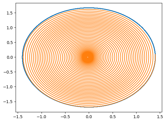
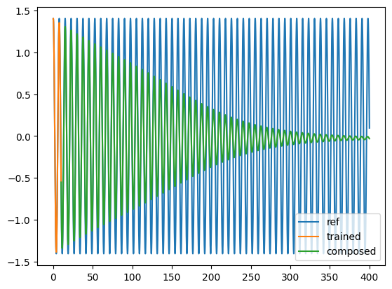
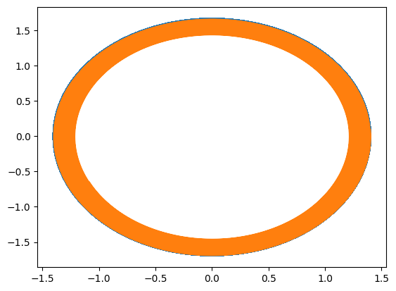
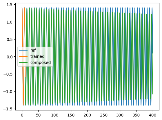
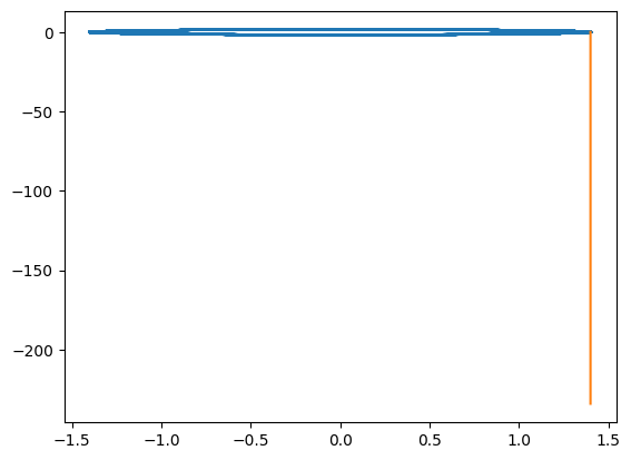
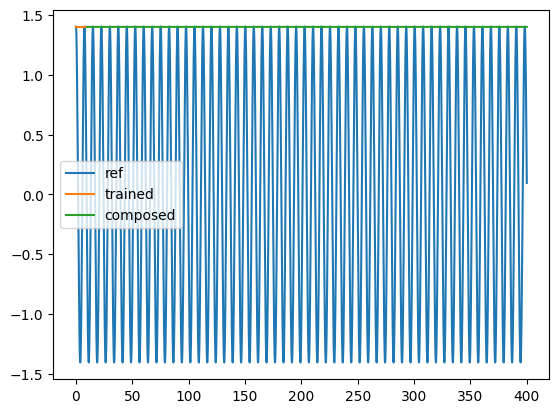
print("#1: Learn the flow with a MLP")

trainer_type = NaturalGradientFlowTrainer if use_natural_gradient else FlowTrainer
epochs = 200 if use_natural_gradient else 5000

space0 = DiscreteFlowSpace(
    2, 1, flow_type=NeuralFlow, net_type=GenericMLP, layer_sizes=[21] * 3, rollout=1
)
print("nb dof: ", space0.ndof)
trainer0 = trainer_type(space0, data)
trainer0.solve(epochs=epochs, batch_size=100, verbose=False)

plt.plot(yref[0, 0, :, 0], yref[0, 0, :, 1])
solution0 = space0.inference(x_testref[0, :][None,], mu_testref[0, :][None,], Nt)
plt.plot(solution0[:, 0, 0].detach().cpu(), solution0[:, 0, 1].detach().cpu())
plt.show()

t = torch.linspace(0, Nt * dt, Nt)

plt.plot(t[:-1], yref[0, 0, :, 0], label="ref")
plt.plot(t[:Nt_train], solution0[:Nt_train, 0, 0].detach().cpu(), label="trained")
plt.plot(
    t[Nt_train - 1 : -1],
    solution0[Nt_train - 1 : -1, 0, 0].detach().cpu(),
    label="composed",
)
plt.legend()
plt.show()

# %%

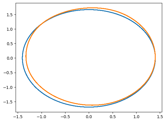
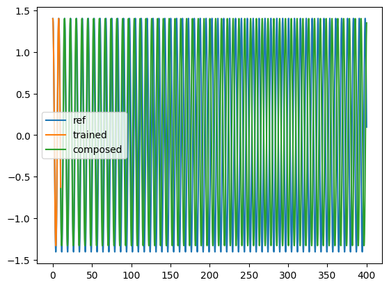
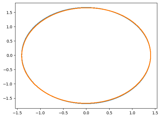
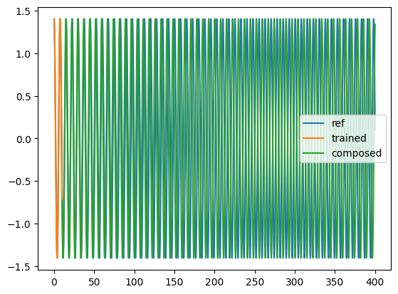
print("#2: Learn the flow with a SympNet")

trainer_type = NaturalGradientFlowTrainer if use_natural_gradient else FlowTrainer
epochs = 200 if use_natural_gradient else 5000

space = DiscreteFlowSpace(
    2, 1, flow_type=NeuralFlow, net_type=SympNet, layer_sizes=[31] * 3, rollout=1
)
trainer = trainer_type(space, data)
trainer.solve(epochs=epochs, batch_size=100, verbose=False)

plt.plot(yref[0, 0, :, 0], yref[0, 0, :, 1])
solution = space.inference(x_testref[0, :][None,], mu_testref[0, :][None,], Nt)
plt.plot(solution[:, 0, 0].detach().cpu(), solution[:, 0, 1].detach().cpu())
plt.show()

t = torch.linspace(0, Nt * dt, Nt)

plt.plot(t[:-1], yref[0, 0, :, 0], label="ref")
plt.plot(t[:Nt_train], solution[:Nt_train, 0, 0].detach().cpu(), label="trained")
plt.plot(
    t[Nt_train - 1 : -1],
    solution[Nt_train - 1 : -1, 0, 0].detach().cpu(),
    label="composed",
)
plt.legend()
plt.show()

# %%

print("#3: Learn an explicit Euler discretization of the flow with a MLP")

trainer_type = NaturalGradientFlowTrainer if use_natural_gradient else FlowTrainer
epochs = 200 if use_natural_gradient else 5000

space2 = DiscreteFlowSpace(
    2,
    1,
    flow_type=ExplicitEulerFlow,
    net_type=GenericMLP,
    layer_sizes=[21] * 3,
    dt=0.02,
    rollout=1,
)
print("nb dof: ", space2.ndof)
trainer2 = trainer_type(space2, data)
trainer2.solve(epochs=epochs, batch_size=100, verbose=False)

plt.plot(yref[0, 0, :, 0], yref[0, 0, :, 1])
solution2 = space2.inference(x_testref[0, :][None,], mu_testref[0, :][None,], Nt)
plt.plot(solution2[:, 0, 0].detach().cpu(), solution2[:, 0, 1].detach().cpu())
plt.show()

t = torch.linspace(0, Nt * dt, Nt)

plt.plot(t[:-1], yref[0, 0, :, 0], label="ref")
plt.plot(t[:Nt_train], solution2[:Nt_train, 0, 0].detach().cpu(), label="trained")
plt.plot(
    t[Nt_train - 1 : -1],
    solution2[Nt_train - 1 : -1, 0, 0].detach().cpu(),
    label="composed",
)
plt.legend()
plt.show()

# %%

print(
    "#4: Learn a symplectic Euler discretization of the flow"
    + "(seen as a Hamiltonian flow) with a MLP"
)

trainer_type = NaturalGradientFlowTrainer if use_natural_gradient else FlowTrainer
epochs = 200 if use_natural_gradient else 5000

space3 = DiscreteFlowSpace(
    2,
    1,
    flow_type=SymplecticEulerFlowSep,
    net_type=GenericMLP,
    layer_sizes=[18] * 3,
    dt=0.02,
    rollout=1,
)
print("nb dof: ", space3.ndof)
trainer3 = trainer_type(space3, data)
trainer3.solve(epochs=epochs, batch_size=100, verbose=False)

plt.plot(yref[0, 0, :, 0], yref[0, 0, :, 1])
solution3 = space3.inference(x_testref[0, :][None,], mu_testref[0, :][None,], Nt)
plt.plot(solution3[:, 0, 0].detach().cpu(), solution3[:, 0, 1].detach().cpu())
plt.show()

t = torch.linspace(0, Nt * dt, Nt)

plt.plot(t[:-1], yref[0, 0, :, 0], label="ref")
plt.plot(t[:Nt_train], solution3[:Nt_train, 0, 0].detach().cpu(), label="trained")
plt.plot(
    t[Nt_train - 1 : -1],
    solution3[Nt_train - 1 : -1, 0, 0].detach().cpu(),
    label="composed",
)
plt.legend()
plt.show()

# %%

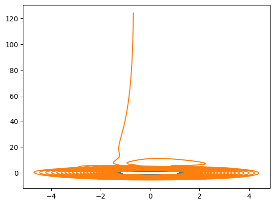
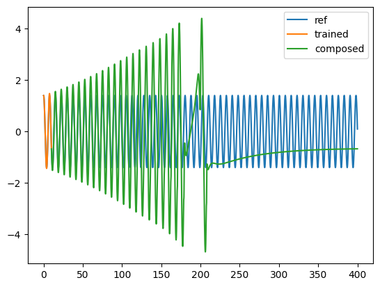
print("#5: Learn the flow with an invertible network")

trainer_type = NaturalGradientFlowTrainer if use_natural_gradient else FlowTrainer
epochs = 200 if use_natural_gradient else 5000

space4 = DiscreteFlowSpace(
    2,
    1,
    flow_type=NeuralFlow,
    net_type=InvertibleNet,
    nb_layers=4,
    layer_sizes=[12] * 2,
    rollout=1,
)
print("nb dof: ", space4.ndof)
trainer4 = trainer_type(space4, data)
trainer4.solve(epochs=epochs, batch_size=100, verbose=False)

plt.plot(yref[0, 0, :, 0], yref[0, 0, :, 1])
solution4 = space4.inference(x_testref[0, :][None,], mu_testref[0, :][None,], Nt)
plt.plot(solution4[:, 0, 0].detach().cpu(), solution4[:, 0, 1].detach().cpu())
plt.show()

t = torch.linspace(0, Nt * dt, Nt)

plt.plot(t[:-1], yref[0, 0, :, 0], label="ref")
plt.plot(t[:Nt_train], solution4[:Nt_train, 0, 0].detach().cpu(), label="trained")
plt.plot(
    t[Nt_train - 1 : -1],
    solution4[Nt_train - 1 : -1, 0, 0].detach().cpu(),
    label="composed",
)
plt.legend()
plt.show()

# %%

print(
    "#6: Learn an explicit Euler discretization of the flow"
    + "(seen as a Hamiltonian flow) with a MLP"
)

trainer_type = NaturalGradientFlowTrainer if use_natural_gradient else FlowTrainer
epochs = 200 if use_natural_gradient else 5000


def potential(x, mu):
    return 0.5 * mu[0] * x[0] ** 2.0 + mu[0] * 0.012 * x[0] ** 3 / 3.0


space5 = DiscreteFlowSpace(
    2,
    1,
    flow_type=ExplicitEulerHamiltonianFlow,
    net_type=GenericMLP,
    layer_sizes=[10] * 3,
    dt=0.02,
    analytic_h=potential,
    rollout=1,
)
print("nb dof: ", space5.ndof)
trainer5 = trainer_type(space5, data)
trainer5.solve(epochs=epochs, batch_size=100, verbose=False)

plt.plot(yref[0, 0, :, 0], yref[0, 0, :, 1])
solution5 = space5.inference(x_testref[0, :][None,], mu_testref[0, :][None,], Nt)
plt.plot(solution5[:, 0, 0].detach().cpu(), solution5[:, 0, 1].detach().cpu())
plt.show()

t = torch.linspace(0, Nt * dt, Nt)

plt.plot(t[:-1], yref[0, 0, :, 0], label="ref")
plt.plot(t[:Nt_train], solution5[:Nt_train, 0, 0].detach().cpu(), label="trained")
plt.plot(
    t[Nt_train - 1 : -1],
    solution5[Nt_train - 1 : -1, 0, 0].detach().cpu(),
    label="composed",
)
plt.legend()
plt.show()

#1: Learn the flow with a MLP
nb dof:  1050
Training: 100%|||||||||||||||||| 200/200[00:05<00:00] , loss: 1.7e+00 -> 2.3e-09

#2: Learn the flow with a SympNet
Training: 100%|||||||||||||||||| 200/200[00:07<00:00] , loss: 1.1e+01 -> 1.5e-07

#3: Learn an explicit Euler discretization of the flow with a MLP
nb dof:  1050
Training: 100%|||||||||||||||||| 200/200[00:05<00:00] , loss: 9.2e-04 -> 3.9e-10

#4: Learn a symplectic Euler discretization of the flow(seen as a Hamiltonian flow) with a MLP
nb dof:  1512
Training: 100%|||||||||||||||||| 200/200[00:13<00:00] , loss: 1.0e-03 -> 1.2e-07

#5: Learn the flow with an invertible network
nb dof:  1632
Training: 100%|||||||||||||||||| 200/200[00:16<00:00] , loss: 3.2e-01 -> 4.1e-04

#6: Learn an explicit Euler discretization of the flow(seen as a Hamiltonian flow) with a MLP
nb dof:  270
Training: 100%|||||||||||||||||| 200/200[00:01<00:00] , loss: 6.3e-04 -> 1.4e-07