Strong boundary conditions

In this second tutorial, we will see how to approximate the solution of the Laplacian problem of the previous tutorials using a PINN with strong boundary condition.

In the following, we implement a PINN with weak boundary condition:

import torch

from scimba_torch.approximation_space.nn_space import NNxSpace
from scimba_torch.domain.meshless_domain.domain_2d import Square2D
from scimba_torch.integration.monte_carlo import DomainSampler, TensorizedSampler
from scimba_torch.integration.monte_carlo_parameters import UniformParametricSampler
from scimba_torch.neural_nets.coordinates_based_nets.mlp import GenericMLP
from scimba_torch.numerical_solvers.elliptic_pde.pinns import (
    NaturalGradientPinnsElliptic,
)
from scimba_torch.physical_models.elliptic_pde.laplacians import (
    Laplacian2DDirichletStrongForm,
)
from scimba_torch.utils.scimba_tensors import LabelTensor

torch.manual_seed(0)

domain_x = Square2D([(0.0, 1), (0.0, 1)], is_main_domain=True)

domain_mu = [(1.0, 2.0)]

sampler = TensorizedSampler(
    [DomainSampler(domain_x), UniformParametricSampler(domain_mu)]
)


def f_rhs(xs: LabelTensor, ms: LabelTensor) -> torch.Tensor:
    x, y = xs.get_components()
    mu = ms.get_components()
    pi = torch.pi
    return 2 * (2.0 * mu * pi) ** 2 * torch.sin(2.0 * pi * x) * torch.sin(2.0 * pi * y)


def f_bc(xs: LabelTensor, ms: LabelTensor) -> torch.Tensor:
    x, _ = xs.get_components()
    return x * 0.0


space = NNxSpace(
    1,  # the output dimension
    1,  # the parameter's space dimension
    GenericMLP,  # the type of neural network
    domain_x,  # the geometric domain
    sampler,  # the sampler
    layer_sizes=[64],  # the size of intermediate layers
)

pde = Laplacian2DDirichletStrongForm(space, f=f_rhs, g=f_bc)

pinn = NaturalGradientPinnsElliptic(pde, bc_type="weak")
pinn.solve(epochs=200, n_collocation=1000, n_bc_collocation=1000, verbose=False)

In order to implement a PINN with strong boundary condition, one approximate the solution \(u\) with a function \(u_{\theta}\) that satisfies the boundary conditions for all \(\theta\).

To this end, one must define a post_processing function that will be applied to the output of the Neural Network (NN) implementing \(u_{\theta}\):

def post_processing(
    inputs: torch.Tensor,  # the output of the NN evaluated at xy, mu
    xy: LabelTensor,
    mu: LabelTensor,
) -> torch.Tensor:
    x, y = xy.get_components()
    return inputs * x * (1.0 - x) * y * (1.0 - y)

the output of this function vanishes on the boundary of \(\Omega\) which is here \([0,1]\times[0,1]\).

Once this function is defines, it is given as an argument to the approximation space implementing \(u_{\theta}\):

space2 = NNxSpace(
    1,  # the output dimension
    1,  # the parameter's space dimension
    GenericMLP,  # the type of neural network
    domain_x,  # the geometric domain
    sampler,  # the sampler
    layer_sizes=[64],  # the size of intermediate layers
    post_processing=post_processing,  # the post-processing function
)

pde2 = Laplacian2DDirichletStrongForm(space2, f=f_rhs, g=f_bc)

This is enough if one wants to compute an approximation with a PINN using classical ADAM, gradient descent or LBFGS optimization algorithm to minimize the residue.

In order to use natural gradient descent algorithms as Energy Natural Gradient or Anagram one has to provide the post-processing function as a function that can be vmapped with torch.func.vmap:

from typing import Callable


def functional_post_processing(
    u: Callable,  # the approximation u
    # u(xy, mu, theta) is a (1,) shaped tensor
    xy: torch.Tensor,  # xy as a torch tensor of shape (2,)
    mu: torch.Tensor,  # mu as a torch tensor of shape (1,)
    theta: torch.Tensor,  # the parameters theta of the approximation space
) -> torch.Tensor:
    return u(xy, mu, theta) * xy[0] * (1.0 - xy[0]) * xy[1] * (1.0 - xy[1])

where the argument u is a functional version of the approximation function, depending on xy, mu and the parameters theta such as:

def u(xy: torch.Tensor, mu: torch.Tensor, theta: torch.Tensor) -> torch.Tensor: ...

that returns the evaluation of the numerical approximation u at non-batched value (xy,mu) for parameters theta. The latter has not to be implemented, it is crafted by Scimba.

When writting the functional post processing, it is important to keep in mind that it will be vmapped for all the variables except theta. As a consequence, it is implemented as a function taking in input non-batched physical variables; for instance here, input xy has shape (2,) as \(\Omega\) has dimension 2.

It has to return a torch tensor of shape (m,) where m is the number of equations of the residual, here 1.

It will be transformed in a batched function during the torch vectorialization process.

Finally, this function has to be given as an argument to the PINN:

pinn2 = NaturalGradientPinnsElliptic(
    pde2,  # the pde
    bc_type="strong",  # specify the strong boundary condition
    # the functional post-processing function
    functional_post_processing=functional_post_processing,
)
pinn2.solve(epochs=200, n_collocation=1000, verbose=False)

import matplotlib.pyplot as plt

from scimba_torch.plots.plots_nd import plot_abstract_approx_spaces


def exact_sol(xs: LabelTensor, ms: LabelTensor) -> torch.Tensor:
    x, y = xs.get_components()
    mu = ms.get_components()
    pi = torch.pi
    return mu * torch.sin(2.0 * pi * x) * torch.sin(2.0 * pi * y)


plot_abstract_approx_spaces(
    (pinn.space, pinn2.space),  # the approximation spaces
    domain_x,  # the spatial domain
    domain_mu,  # the parameter's domain
    loss=(pinn.losses, pinn2.losses),  # optional plot of the loss: the losses
    error=exact_sol,  # optional plot of the approximation error: the exact solution
    draw_contours=True,  # plotting isolevel lines
    n_drawn_contours=20,  # number of isolevel lines,
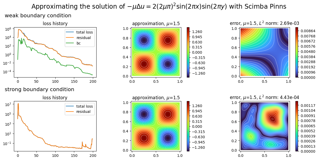
    title=(
        "Approximating the solution of "
        r"$- \mu\Delta u = 2(2\mu\pi)^2 \sin(2\pi x) \sin(2\pi y)$"
        " with Scimba Pinns"
    ),
    titles=("weak boundary condition", "strong boundary condition"),
)
plt.show()