Scimba basics II: Natural gradient preconditioners

In the previous tutorials, we used a PINN fit through a natural gradient descent algorithm to the solution of a 2D laplacian problem.

Scimba implements two natural gradient preconditioners for gradient descent algorithms: Energy Natural Gradient (ENG) and Anagram.

Both can be used for PINNs and the task of projecting a function onto an approximation space.

This tutorial demonstrates further the use of ENG and Anagram preconditioners in Scimba for PINNs on the 2D laplacian example, and for projectors. A following tutorial explains how to model a pde so that it can be used with a natural gradient preconditioned PINN.

Let us first define the problem we consider, and solve it with a not preconditioned PINN for the reference.

Approximation with a not preconditioned PINN

import torch

from scimba_torch.approximation_space.nn_space import NNxSpace
from scimba_torch.domain.meshless_domain.domain_2d import Square2D
from scimba_torch.integration.monte_carlo import DomainSampler, TensorizedSampler
from scimba_torch.integration.monte_carlo_parameters import UniformParametricSampler
from scimba_torch.neural_nets.coordinates_based_nets.mlp import GenericMLP
from scimba_torch.physical_models.elliptic_pde.laplacians import (
    Laplacian2DDirichletStrongForm,
)
from scimba_torch.utils.scimba_tensors import LabelTensor

torch.manual_seed(0)

domain_x = Square2D([(0.0, 1), (0.0, 1)], is_main_domain=True)

domain_mu = [(0.5, 1.0)]

sampler = TensorizedSampler(
    [DomainSampler(domain_x), UniformParametricSampler(domain_mu)]
)

def f_rhs(xs: LabelTensor, ms: LabelTensor) -> torch.Tensor:
    x, y = xs.get_components()
    mu = ms.get_components()
    pi = torch.pi
    return 2 * (2.0 * mu * pi) ** 2 * torch.sin(2.0 * pi * x) * torch.sin(2.0 * pi * y)

def f_bc(xs: LabelTensor, ms: LabelTensor) -> torch.Tensor:
    x, _ = xs.get_components()
    return x * 0.0

space = NNxSpace(
    1,  # the output dimension
    1,  # the parameter's space dimension
    GenericMLP,  # the type of neural network
    domain_x,  # the geometric domain
    sampler,  # the sampler
    layer_sizes=[16, 16],  # the size of intermediate layers
)

pde = Laplacian2DDirichletStrongForm(space, f=f_rhs, g=f_bc)

We define a PinnsElliptic object to approximate the solution of pde.

Notice the use of keyword argument bc_weight to scale the loss induced by the boundary condition relatively to the loss of the residual inside the domain.

from scimba_torch.numerical_solvers.elliptic_pde.pinns import PinnsElliptic

pinn = PinnsElliptic(pde, # the pde to be solved
                     bc_type="weak", # use explicitly the boundary conditions
                     bc_weight=50.) # the weight of the loss of the boundary condition

The next step is to solve the PINN, that is to find the parameters of the approximation space (here a multi-layer perceptron) to minimize the residual inside the domain and the boundary condition, here Dirichlet.

At each step, this requires to sample the interior and the boundaries of the considered domain \(\Omega\). Below, we time 1000 steps of the Adam optimizer.

import timeit

start = timeit.default_timer()
pinn.solve(epochs=1000, #number of steps of optimization
           n_collocation=1000, #number of sample points inside the domain
           n_bc_collocation=1000, #number of sample points on the boundary
           verbose=False)
end = timeit.default_timer()

print("time in approximation with a PINN: ", end - start)
print("best loss: ", pinn.best_loss)

time in approximation with a PINN:  4.099338083062321
best loss:  18.456674964641266

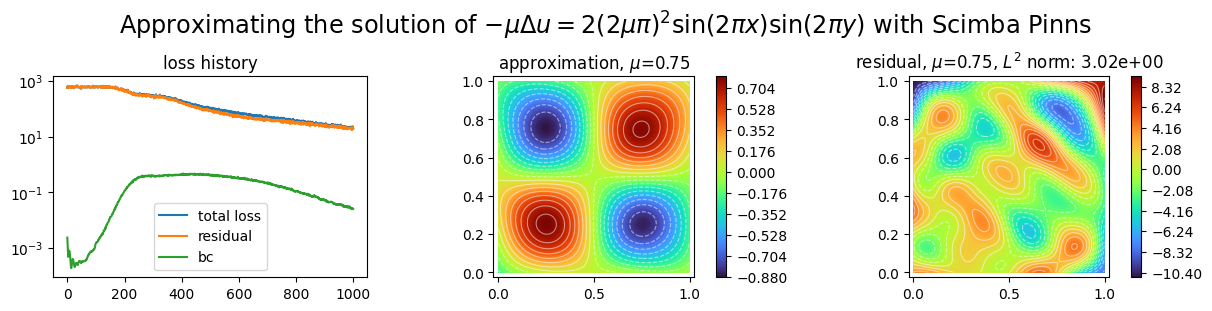
Let us plot the obtained approximation, the residual inside the domain and the history of the loss variation during the optimization.

import matplotlib.pyplot as plt

from scimba_torch.plots.plots_nd import plot_abstract_approx_spaces

plot_abstract_approx_spaces(
    pinn.space,  # the approximation space
    domain_x,  # the spatial domain
    domain_mu,  # the parameter's domain
    loss=pinn.losses,  # optional plot of the loss: the losses
    residual=pinn.pde,  # optional plot of the residual of the pde
    draw_contours=True,  # plotting isolevel lines
    n_drawn_contours=20,  # number of isolevel lines,
    title=(
        "Approximating the solution of "
        r"$- \mu\Delta u = 2(2\mu\pi)^2 \sin(2\pi x) \sin(2\pi y)$"
        " with Scimba Pinns"
    ),
)
plt.show()

Approximation with preconditioned PINNs

Scimba implements two natural gradient descent algorithms for PINNs: Energy Natural Gradient and Anagram.

For linear PDEs (as is the laplacian equation under consideration), both approaches rely on pseudo inverting the so called energy Gram matrix, however the numerical methods used to do so differ.

Energy Natural Gradient preconditioning

ENGspace = NNxSpace(
    1,  # the output dimension
    1,  # the parameter's space dimension
    GenericMLP,  # the type of neural network
    domain_x,  # the geometric domain
    sampler,  # the sampler
    layer_sizes=[16, 16],  # the size of intermediate layers
)

ENGpde = Laplacian2DDirichletStrongForm(ENGspace, f=f_rhs, g=f_bc)

PINNs with ENG descent algorithm are NaturalGradientPinnsElliptic objects.

Notice the use of the matrix_regularization argument when instantiating the pinn. It is set to \(10^{-6}\) by default which suits to most problems.

from scimba_torch.numerical_solvers.elliptic_pde.pinns import (
    NaturalGradientPinnsElliptic,
)

ENGpinn = NaturalGradientPinnsElliptic(ENGpde,
                                       bc_type="weak",
                                       bc_weight=50.,
                                       matrix_regularization=1e-6)

Use SGD algorithm together with a line search for adaptive choice of learning rate.

start = timeit.default_timer()
ENGpinn.solve(epochs=200,
              n_collocation=1000,
              n_bc_collocation=1000,
              verbose=False)
end = timeit.default_timer()

print("time in approximation with ENG preconditioned PINN: ", end - start)
print("best loss: ", ENGpinn.best_loss)

time in approximation with ENG preconditioned PINN:  4.473929750034586
best loss:  9.994778387640557e-05

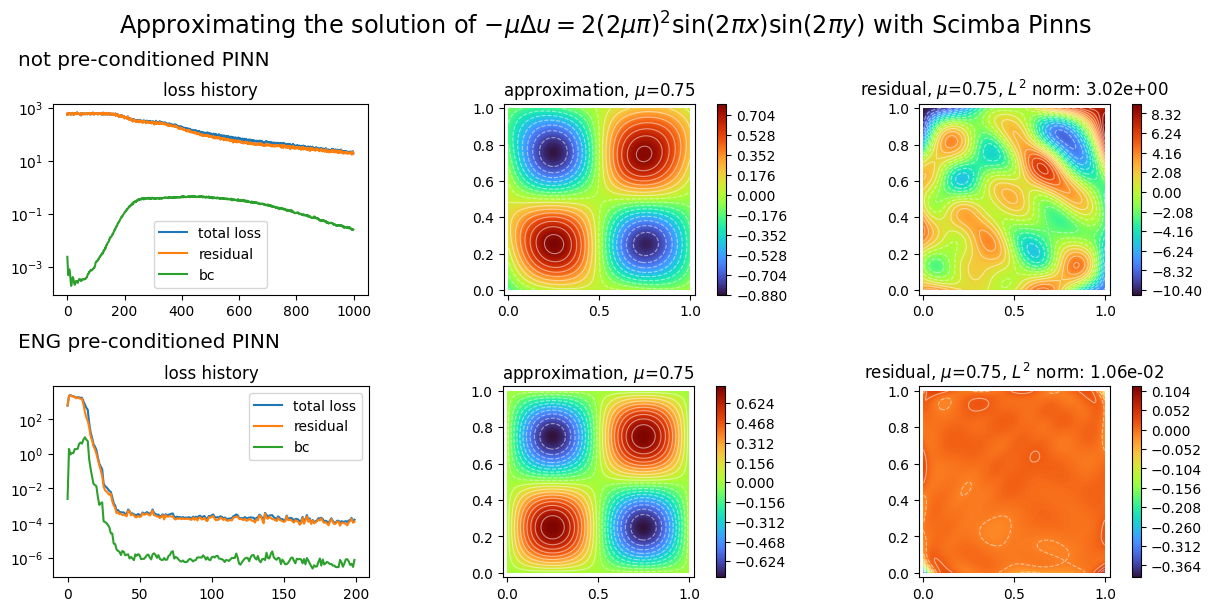
We plot the two PINNs with:

plot_abstract_approx_spaces(
    (pinn.space, ENGpinn.space),  # the approximation spaces
    domain_x,  # the spatial domain
    domain_mu,  # the parameter's domain
    loss=(pinn.losses, ENGpinn.losses),  # optional plot of the loss: the losses
    residual=(pinn.pde, ENGpinn.pde),  # optional plot of the residual of the pde
    draw_contours=True,  # plotting isolevel lines
    n_drawn_contours=20,  # number of isolevel lines,
    title=(
        "Approximating the solution of "
        r"$- \mu\Delta u = 2(2\mu\pi)^2 \sin(2\pi x) \sin(2\pi y)$"
        " with Scimba Pinns"
    ),
    titles=("not preconditioned PINN", "ENG preconditioned PINN"),
)
plt.show()

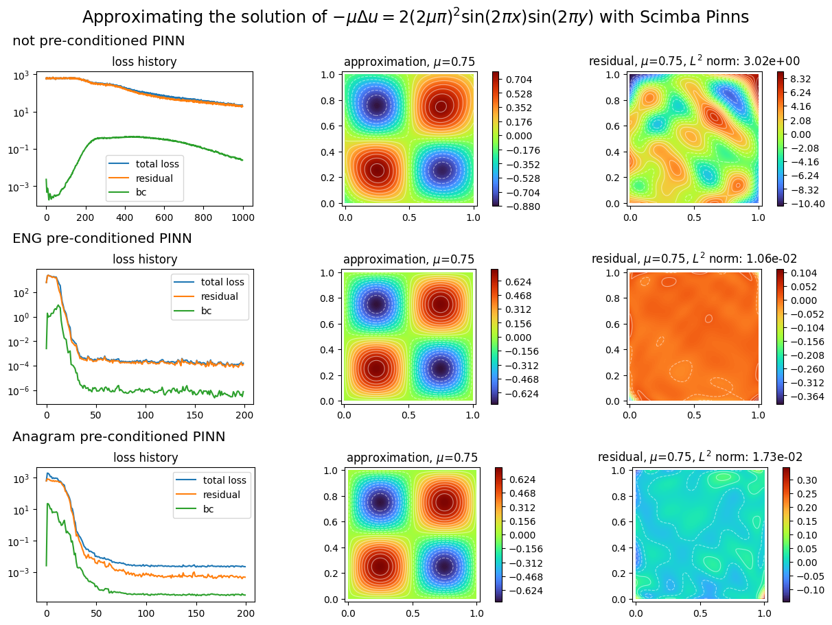
Anagram preconditioning

In order to demonstrate Anagram use, we define new approximation space and PDE:

ANAspace = NNxSpace(
    1,  # the output dimension
    1,  # the parameter's space dimension
    GenericMLP,  # the type of neural network
    domain_x,  # the geometric domain
    sampler,  # the sampler
    layer_sizes=[16, 16],  # the size of intermediate layers
)

ANApde = Laplacian2DDirichletStrongForm(ANAspace, f=f_rhs, g=f_bc)

PINNs with Anagram gradient descent algorithm are AnagramPinnsElliptic objects.

Notice the use below of the svd_threshold argument when creating the AnagramPinnsElliptic object. The success of the optimization is very sensitive to this parameter; its default value of \(10^{-6}\) might be a very bad choice for some examples.

from scimba_torch.numerical_solvers.elliptic_pde.pinns import AnagramPinnsElliptic

ANApinn = AnagramPinnsElliptic(
    ANApde, bc_type="weak", bc_weight=50.0, svd_threshold=0.1
)

start = timeit.default_timer()
ANApinn.solve(epochs=200, n_collocation=1000, n_bc_collocation=1000, verbose=False)
end = timeit.default_timer()

print("time in approximation with Anagram preconditioned PINN: ", end - start)
print("best loss: ", ANApinn.best_loss)

plot_abstract_approx_spaces(
    (pinn.space, ENGpinn.space, ANApinn.space),  # the approximation space
    domain_x,  # the spatial domain
    domain_mu,  # the parameter's domain
    loss=(
        pinn.losses,
        ENGpinn.losses,
        ANApinn.losses,
    ),  # optional plot of the loss: the losses
    residual=(
        pinn.pde,
        ENGpinn.pde,
        ANApinn.pde,
    ),  # optional plot of the residual of the pde
    draw_contours=True,  # plotting isolevel lines
    n_drawn_contours=20,  # number of isolevel lines,
    title=(
        "Approximating the solution of "
        r"$- \mu\Delta u = 2(2\mu\pi)^2 \sin(2\pi x) \sin(2\pi y)$"
        " with Scimba Pinns"
    ),
    titles=(
        "not preconditioned PINN",
        "ENG preconditioned PINN",
        "Anagram preconditioned PINN",
    ),
)
plt.show()

time in approximation with Anagram preconditioned PINN:  10.302835624897853
best loss:  0.002102398089162228

We explain in this tutorial how to write a model for which natural gradient preconditioners can be used.

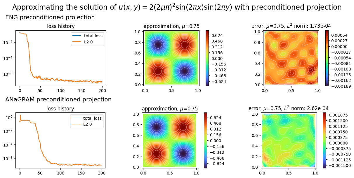
preconditioned projectors

To finish with, we show how to project a known function on an approximation space with preconditioned gradient descent optimization. We project the exact solution the 2D laplacian problem considered so far.

from scimba_torch.numerical_solvers.collocation_projector import (
    NaturalGradientProjector,
)


def exact_sol(xs: LabelTensor, ms: LabelTensor) -> torch.Tensor:
    x, y = xs.get_components()
    mu = ms.get_components()
    pi = torch.pi
    return mu * torch.sin(2.0 * pi * x) * torch.sin(2.0 * pi * y)


ENGspace = NNxSpace(1, 1, GenericMLP, domain_x, sampler, layer_sizes=[16, 16])

ENGprojector = NaturalGradientProjector(ENGspace, exact_sol)

start = timeit.default_timer()
ENGprojector.solve(epochs=200, n_collocation=2000, verbose=False)
end = timeit.default_timer()
print("time in projection with ENG preconditioning: ", end - start)
print("best L2 error: ", ENGprojector.best_loss)

ANAspace = NNxSpace(1, 1, GenericMLP, domain_x, sampler, layer_sizes=[16, 16])

ANAprojector = NaturalGradientProjector(ANAspace, exact_sol)

start = timeit.default_timer()
ANAprojector.solve(epochs=200, n_collocation=2000, verbose=False)
end = timeit.default_timer()
print("time in projection with Anagram preconditioning: ", end - start)
print("best L2 error: ", ANAprojector.best_loss)

time in projection with ENG preconditioning:  1.50338145904243
best L2 error:  3.799797998913824e-08
time in projection with Anagram preconditioning:  1.4730335830245167
best L2 error:  6.021763265951982e-08

plot_abstract_approx_spaces(
    (ENGprojector.space, ANAprojector.space),  # the approximation space
    domain_x,  # the spatial domain
    domain_mu,  # the parameter's domain
    # optional plot of the loss: the losses
    loss=(ENGprojector.losses, ANAprojector.losses),
    error=exact_sol,  # plot the error w.r.t. the exact solution
    draw_contours=True,  # plotting isolevel lines
    n_drawn_contours=20,  # number of isolevel lines,
    title=(
        "Approximating the solution of "
        r"$u(x,y) = 2(2\mu\pi)^2 \sin(2\pi x) \sin(2\pi y)$"
        " with preconditioned projection"
    ),
    titles=("ENG preconditioned projection", "Anagram preconditioned projection"),
)
plt.show()