Creating meshless domains

In this tutorial we will see how to:

• Create a simple Domain

• Apply a mapping to a Domain

• Create a Domain with holes

• Create sub-domains

• Defining your own Domains with a custom Signed Distance Function

• Available domain showcase

• Using the threshold to avoid sampling near the boundary

# import necessary libraries
import matplotlib.pyplot as plt
import torch

Some general geometries in 1D, 2D and 3D are already implemented.

# import classical domains
from scimba_torch.domain.meshless_domain import (
    Cube3D,
    Cylinder3D,
    Disk2D,
    Disk3D,
    Polygon2D,
    Segment1D,
    Square2D,
    Torus3D,
    TorusFrom2DVolume,
)

Creating a simple Domain

To create a simple domain, simply instantiate one of the meshless_domain class with the appropriate parameters.

The flag is_main_domain is used to specify if the domain can have subdomains/holes.

It is not mandatory to set it to true but strongly advised, as general samplers are designed to work on main domains only.

square = Square2D(
    bounds=[(-1, 1), (0, 1)],
    is_main_domain=True
)

# to reset the square domain
def simple_square():
    return Square2D(
        bounds=[(-1, 1), (0, 1)],
        is_main_domain=True
    )

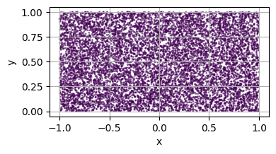
To visualise a domain, we are going to sample points on it

# import necessary libraries
from scimba_torch.integration.monte_carlo import DomainSampler


# a utility function to plot a 2D domain
def plot_2d(domain, n=10_000, ax=None):
    """Plot a 2D domain using a Domain sampler."""

    # create the sampler
    sampler = DomainSampler(domain)

    # sample points
    res = sampler.sample(n)
    pts = res.x         # coordinates of the sampled points
    labels = res.labels # labels of the sampled points

    # convert to numpy for plotting
    pts = pts.detach().cpu().numpy()
    labels = labels.detach().cpu().numpy()

    # generate the ax if not provided
    if ax is None:
        fig = plt.figure(figsize=(4, 4))
        ax = fig.add_subplot(111, xlabel='x', ylabel='y', aspect='equal')
    else:
        fig = None
        ax.set_xlabel('x')
        ax.set_ylabel('y')
        ax.set_aspect('equal')

    # plot the points
    ax.scatter(pts[:, 0], pts[:, 1], s=1, c=labels, alpha=0.5)
    ax.grid(True)

    if fig is not None:
        fig.tight_layout()
        plt.show()

square = simple_square()
plot_2d(square)

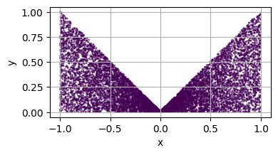
Apply a Mapping to a Domain

We can also consider a mapped domain.

To do so, simply declare a mapping and set it to the domain, specifying a bounding box of the mapped domain.

For more informations about mappings, see Complement on the mapping.

from scimba_torch.utils.mapping import Mapping


# define a mapping function
def map(x):
    """A simple mapping function."""
    # x: (N, 2) tensor
    # out: (N, 2) transformed tensor
    return torch.stack([x[:, 0], x[:, 1]*(torch.abs(x[:, 0]) + 1e-2)], dim=1)

# define the mapping
mapping = Mapping(
    from_dim=2,     # original dimension
    to_dim=2,       # mapped dimension
    map=map,        # mapping function
    inv=None,       # optional inverse mapping function
)

# set the mapping for the square domain
square = simple_square()
square.set_mapping(
    map=mapping,
    bounds_postmap=[(-1, 1), (0, 1)], # bounding box of the MAPPED domain
)

plot_2d(square)

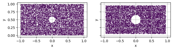
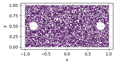
Create a Domain with holes

We can also add holes to a domain.

A hole is a domain as well, defined with the flag is_main_domain set to false.

For example, let’s consider a disk hole inside the domain

square = simple_square()
# create some holes
hole1 = Disk2D(center=(.8, 0.5), radius=0.1, is_main_domain=False)
hole2 = Disk2D(center=(-.8, 0.5), radius=0.1, is_main_domain=False)

# add holes to the square domain
square.add_hole(hole1)
square.add_hole(hole2)

plot_2d(square)

# helper for resetting the domains
def simple_disks():
    disk_L = Disk2D(center=(-.8, 0.5), radius=0.1, is_main_domain=False)
    disk_R = Disk2D(center=(.8, 0.5), radius=0.1, is_main_domain=False)
    return disk_L, disk_R

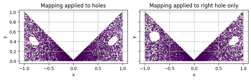
Combining Holes and Mapping

We can also combine holes and mappings.

By default, the mapping is applied to holes as well as the domain.

We can change this behavior when:

• adding a hole (if the mapping is already set), with the flag copy_mapping set to False

• setting the mapping for all already added holes, with the flag to_holes set to False

Yet, we recommend to proceed in the following order:

1. Create the main domain

2. Set the mapping if any

3. Add holes to the domain, with copy_mapping set to False if we do not want to apply the mapping on the hole

fig, axs = plt.subplots(1, 3, figsize=(12, 4), sharex=True, sharey=True)

# by default, the mapping is applied to all the holes
square = simple_square()
disk_L, disk_R = simple_disks()
square.set_mapping(map=mapping, bounds_postmap=[(-1, 1), (0, 1)])
square.add_hole(disk_L)
square.add_hole(disk_R)

# plot
plot_2d(square, ax=axs[0])
axs[0].set_title('Mapping applied to holes')


# we can  specify not to apply the mapping to a specific hole when adding it
square = simple_square()
disk_L, disk_R = simple_disks()
square.set_mapping(map=mapping, bounds_postmap=[(-1, 1), (0, 1)])
square.add_hole(disk_L, copy_mapping=False)
square.add_hole(disk_R, copy_mapping=True)

# plot
plot_2d(square, ax=axs[1])
axs[1].set_title('Mapping applied to right hole only')


# # Alternatively, we can specify not to apply the mapping to already existing holes,
# # but we will prefer to set the mapping first and then add the holes
# square = simple_square()
# disk_L, disk_R = simple_disks()
# square.add_hole(disk_L)
# square.set_mapping(map=mapping, bounds_postmap=[(-1, 1), (0, 1)], to_holes=False)
# square.add_hole(disk_R)

# plot2D(square, ax=axs[2])
# axs[2].set_title('Mapping applied to right hole only')
axs[2].remove()


fig.tight_layout()
plt.show()

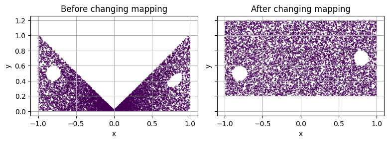
When changing the mapping of the domain (i.e. the domain was already mapped) with the flag to_holes set to False, the mapping will still be applied to previously mapped holes.

fig, axs = plt.subplots(1, 2, figsize=(8, 4), sharex=True, sharey=True)

square = simple_square()
disk_L, disk_R = simple_disks()

# define a new mapping
mapping2 = Mapping.translate(torch.tensor([0, 0.2]))

# set the mapping for the square domain
square.set_mapping(map=mapping, bounds_postmap=[(-1, 1), (0, 1)])

# add the holes
square.add_hole(disk_L, copy_mapping=False) # left hole WITHOUT mapping
square.add_hole(disk_R)                     # right hole with mapping

# plot
plot_2d(square, ax=axs[0])
axs[0].set_title("Before changing mapping")

# apply the new mapping to the square domain
square.set_mapping(map=mapping2, bounds_postmap=[(-1, 1), (0.2, 1.2)], to_holes=False)

# plot
plot_2d(square, ax=axs[1])
axs[1].set_title("After changing mapping\n(previously mapped holes get new mapping)")

fig.tight_layout()
plt.show()

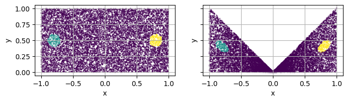
Create sub-domains

We can add subdomains to a main domain. This will give a label specific to which subdomain does the point belong

Unlike the holes, a mapping applied to a domain is always applied on subdomains.

fig, axs = plt.subplots(1, 2, figsize=(8, 4), sharex=True, sharey=True)


square = simple_square()
disk_L, disk_R = simple_disks()
square.add_subdomain(disk_L)
square.add_subdomain(disk_R)

plot_2d(square, ax=axs[0])

square.set_mapping(map=mapping, bounds_postmap=[(-1, 1), (0, 1)])
plot_2d(square, ax=axs[1])

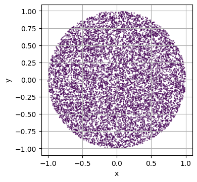
Defining your own Domains with a custom Signed Distance Function

In Scimba, domain are defined with a signed distance function and a bounding box.

A Domain should inherit from VolumetricDomain

A Signed distance function is simply a Callable with a threshold

# import necessary libraries
from scimba_torch.domain.meshless_domain.base import VolumetricDomain
from scimba_torch.domain.sdf import SignedDistance


class CustomSDF(SignedDistance):
    """A custom SDF class that defines the signed distance function for unit 2D disk."""

    def __init__(self):
        super().__init__(
            dim=2,
            threshold=0.0,      # threshold for inside points (sdf < -threshold)
            threshold_out=0.0,  # threshold for outside points, use for holes (sdf > threshold_out)
        )

    def __call__(self, pts: torch.Tensor) -> torch.Tensor:
        """Compute the signed distance function for the unit 2D disk."""
        # pts: (N, dim) tensor
        x, y = pts[:, 0], pts[:, 1]
        return (torch.sqrt(x**2 + y**2) - 1.0)[:, None]  # out: (N, 1) tensor


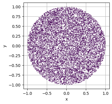
custom_domain = VolumetricDomain(
    domain_type="CustomUnitDisk",
    dim=2,
    sdf=CustomSDF(),
    bounds=[(-1, 1), (-1, 1)],
    is_main_domain=True,
)

plot_2d(custom_domain)

/var/folders/zp/w4p46p_n0p52lgf7h0vpbrt00000gn/T/ipykernel_40294/3476767848.py:10: UserWarning: The domain does not have boundary domains
  sampler = DomainSampler(domain)

Boundary Domains

TODO : implement default sampling with sdf when no bc domains are given ?

As you can see in the last example, our custom domain does not have any boundary domains…

In Scimba boundary domain (more generally called SurfacicDomains), are a “proper” domain (i.e. a VolumetricDomain) of dimension \(d\), mapped to dimension \(d+1\)

To declare such a domain, we hence need:

• A VolumetricDomain (called parametric_domain)

• A Mapping (called surface) that embeds our parametric_domain into higher dimension.

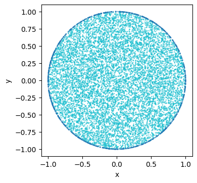
Let’s define the boundary of our unit disk.

# import necessary libraries
from scimba_torch.domain.meshless_domain.base import SurfacicDomain

bc = SurfacicDomain(
    domain_type="CustomUnitCircle",
    parametric_domain=Segment1D((0, 2 * torch.pi)),
    surface=Mapping(
        from_dim=1,
        to_dim=2,
        map=lambda x: torch.stack([torch.cos(x[..., 0]), torch.sin(x[..., 0])], dim=-1),
    ),
)

# we then add the boundary domain to our custom domain
custom_domain.add_bc_domain(bc)

# we don't have a warning anymore :)
plot_2d(custom_domain)

Let’s create a new plotting utility function to see what’s happening.

# a utility function to plot a 2D domain and boundary points
def plot_2d_with_bc(domain, n=10_000, n_bc=1_000, ax=None):
    """Plot a 2D domain using a Domain sampler."""

    cmap = plt.get_cmap("tab10_r")

    # create the sampler
    sampler = DomainSampler(domain)

    # sample points
    res = sampler.sample(n)
    pts = res.x         # coordinates of the sampled points
    labels = res.labels # labels of the sampled points

    # sample boundary points
    res_bc, _ = sampler.bc_sample(n_bc)
    pts_bc = res_bc.x           # coordinates of the sampled boundary points
    labels_bc = res_bc.labels   # labels of the sampled boundary points

    # convert to numpy for plotting
    pts = pts.detach().cpu().numpy()
    labels = labels.detach().cpu().numpy()
    pts_bc = pts_bc.detach().cpu().numpy()
    labels_bc = labels_bc.detach().cpu().numpy()

    # generate the ax if not provided
    if ax is None:
        fig = plt.figure(figsize=(4, 4))
        ax = fig.add_subplot(111, xlabel="x", ylabel="y", aspect="equal")
    else:
        fig = None
        ax.set_xlabel("x")
        ax.set_ylabel("y")
        ax.set_aspect("equal")

    # offset the labels for boundary points
    labels_bc += labels.max() + 1
    max_label = max(labels.max(), labels_bc.max())

    # plot the points
    ax.scatter(
        pts[:, 0],
        pts[:, 1],
        s=1,
        c=labels,
        alpha=0.5,
        cmap=cmap,
        vmin=0,
        vmax=max_label,
    )

    # plot the boundary points
    ax.scatter(
        pts_bc[:, 0],
        pts_bc[:, 1],
        s=1,
        c=labels_bc,
        cmap=cmap,
        vmin=0,
        vmax=max_label,
        alpha=0.5,
    )

    if fig is not None:
        fig.tight_layout()
        plt.show()


plot_2d_with_bc(custom_domain)

!Warning! Be aware that their is not check or whatsoever to see it the given boundary domain is really the boundary of the given domain.

Previously, we did not get any warning because the Square2D domain implements full_bc_domain, which returns a list of SurfacicDomains that represent the boundary of a square.

When no user-specif boundary domains are provided, it defaults to the full_bc_domain.

Complement on the mapping

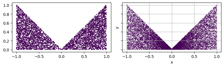
Note that the Mapping can take extra arguments:

• jac to declare the jacobian of the mapping (if not provided, it is computed using torch torch.func.jacrev)

• inv to be declared if the mapping is considered invertible

• inv_jac for the jacobian of the inverse (otherwise computed as jac)

As you should have noticed, once a domain is mapped, the basic sampling will not yield an uniform sampling anymore.

That is because we sample uniformly in the domain before mapping, then apply the mapping.

To still have it you need to declare an invertible mapping and use sample_post_map.

from scimba_torch.integration.monte_carlo import SurfacicSampler, VolumetricSampler


# define a mapping function
def map(x):
    """A simple mapping function."""
    return torch.stack([x[:, 0], x[:, 1]*(torch.abs(x[:, 0]) + 1e-2)], dim=1)

# define the inverse mapping function
def inv(y):
    """Inverse of the mapping function."""
    return torch.stack([y[:, 0], y[:, 1]/(torch.abs(y[:, 0]) + 1e-2)], dim=1)



# define the mapping
mapping = Mapping(
    from_dim=2,
    to_dim=2,
    map=map,
    inv=inv
)

square = simple_square()

# set the mapping for the square domain
square.set_mapping(
    map=mapping,
    bounds_postmap=[(-1, 1), (0, 1)],
)

# create the sampler
sampler = VolumetricSampler(square)

# sample points
pts = sampler.sample_postmap(5_000)
pts = pts.detach().cpu().numpy()

# plot the points
fig, axs = plt.subplots(1, 2, figsize=(8, 4), sharex=True, sharey=True)
axs[0].scatter(pts[:, 0], pts[:, 1], s=1, c=torch.zeros(pts.shape[0]).numpy())
axs[0].set_aspect('equal')

plot_2d(square, ax=axs[1])
fig.tight_layout()
plt.show()

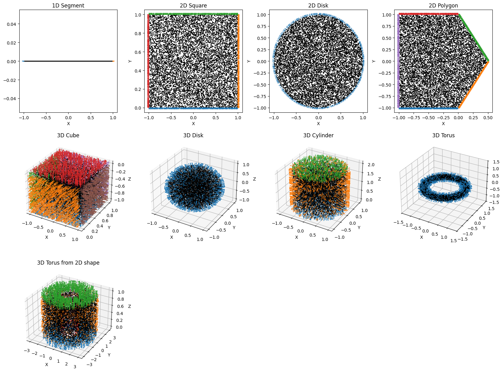
Available domain showcase

# 1D domains
segment = Segment1D(
    low_high=(-1, 1),
    is_main_domain=True
)

# 2D domains
square = Square2D(
    bounds=[(-1, 1), (0, 1)],
    is_main_domain=True
)

disk = Disk2D(
    center=(0, 0),
    radius=1,
    is_main_domain=True
)
polygon = Polygon2D(
    # vertices of the polygon, they should be provided in counter-clockwise order
    vertices=[[-1, -1], [0, -1], [.5, 0], [0, 1], [-1, 1]],
    is_main_domain=True
)

# 3D domains
cube = Cube3D(
    bounds=[(-1, 1), (0, 1), (-1, 0)],
    is_main_domain=True
)
disk3d = Disk3D(
    center=(0, 0, 0),
    radius=1,
    is_main_domain=True
)
cylinder = Cylinder3D(
    radius=1,
    length=2,
    is_main_domain=True
)
torus = Torus3D(
    center=(0, 0, 0),
    radius=1,
    tube_radius=0.2,
    is_main_domain=True
)
torus_from2d = TorusFrom2DVolume(
    base_volume=square,
    radius=2,
    is_main_domain=True
)

# import necessary libraries
from scimba_torch.integration.monte_carlo import VolumetricSampler


# utility function to sample and plot points in a domain
def plot(dict_dom2ax, n=10_000, n_bc=1000):
    for domain, ax in dict_dom2ax.items():
        # create a sampler for the domain
        sampler = VolumetricSampler(domain)
        bc_sampler = [SurfacicSampler(bc) for bc in domain.full_bc_domain()]
        # sample N points
        pts = sampler.sample(n)
        bc_pts = [
            bc_sampler[i].sample(n_bc, compute_normals=True)
            for i in range(len(bc_sampler))
        ]
        # convert to numpy for plotting (& normalize normals)
        pts = pts.detach().numpy()
        bc_pts = [
            (bc, 0.1 * n / torch.linalg.norm(n, axis=-1, keepdims=True))
            for bc, n in bc_pts
        ]
        bc_pts = [(bc[0].detach().numpy(), bc[1].detach().numpy()) for bc in bc_pts]

        def get_pts(pts):
            if domain.dim == 1:
                return pts[:, 0], [0] * len(pts)
            elif domain.dim == 2:
                return pts[:, 0], pts[:, 1]
            elif domain.dim == 3:
                return pts[:, 0], pts[:, 1], pts[:, 2]
            else:
                raise ValueError("Domain dimension not supported for plotting.")

        ax.scatter(*get_pts(pts), color="k", s=1)  # plot the sampled points

        for i, (bc, nn) in enumerate(bc_pts):
            ax.scatter(
                *get_pts(bc), s=1, c=f"C{i}", alpha=0.2
            )  # plot the boundary points
            ax.quiver(
                *get_pts(bc), *get_pts(nn), color=f"C{i}", alpha=0.5
            )  # plot the boundary normals


fig = plt.figure(figsize=(16, 12))
dict_dom2ax = {
    segment: fig.add_subplot(3, 4, 1, xlabel="X", title="1D Segment"),
    square: fig.add_subplot(3, 4, 2, xlabel="X", ylabel="Y", title="2D Square"),
    disk: fig.add_subplot(3, 4, 3, xlabel="X", ylabel="Y", title="2D Disk"),
    polygon: fig.add_subplot(3, 4, 4, xlabel="X", ylabel="Y", title="2D Polygon"),
    cube: fig.add_subplot(
        3, 4, 5, projection="3d", xlabel="X", ylabel="Y", zlabel="Z", title="3D Cube"
    ),
    disk3d: fig.add_subplot(
        3, 4, 6, projection="3d", xlabel="X", ylabel="Y", zlabel="Z", title="3D Disk"
    ),
    cylinder: fig.add_subplot(
        3,
        4,
        7,
        projection="3d",
        xlabel="X",
        ylabel="Y",
        zlabel="Z",
        title="3D Cylinder",
    ),
    torus: fig.add_subplot(
        3,
        4,
        8,
        projection="3d",
        xlabel="X",
        ylabel="Y",
        zlabel="Z",
        xlim=(-1.5, 1.5),
        ylim=(-1.5, 1.5),
        zlim=(-1.5, 1.5),
        title="3D Torus",
    ),
    torus_from2d: fig.add_subplot(
        3,
        4,
        9,
        projection="3d",
        xlabel="X",
        ylabel="Y",
        zlabel="Z",
        title="3D Torus from 2D shape",
    ),
}

# plot the domains
plot(dict_dom2ax)
fig.tight_layout()
plt.show()

Using the threshold to avoid sampling near the boundary

The domains present in scimba are (mostly) implemented using exact signed distance functions.

This means that points sampled with them can be arbitrarily close to the boundary.

To avoid this, you can use set_threshold on a main domain.

This will modified the threshold (resp. threshold_out) of the main domain (resp. holes).

NOTE: the exact distance to the boundary excluded will depend on the specific sdf of each domain.

For finer control, you can use domain.sdf.threshold for the domain and hole.sdf.threshold_out for each hole.

TODO : “uniformize” sdf of domains ?

fig, axs = plt.subplots(1, 2, figsize=(8, 4), sharex=True, sharey=True)

square = simple_square()
hole = Disk2D(center=(0, 0.5), radius=0.1, is_main_domain=False)
square.add_hole(hole)

# plot with default threshold
plot_2d(square, ax=axs[0])

# set a threshold to avoid sampling near the boundary
square.set_threshold(0.05)
plot_2d(square, ax=axs[1])