Scimba basics I: approximation of the solution of a 2D Laplacian

In this first tutorial, we’ll walk you through the basic steps to approximate the solution of a 2D Laplacian Partial Differential Equation (PDE) with a Scimba Physics-Informed Neural Network (PINN).

We consider the equation:

\[- \mu\Delta u = 2(2\mu\pi)^2 \sin(2\pi x) \sin(2\pi y)\]

on \((x,y) \in \Omega := [0, 1]\times[0, 1]\) with parameter \(\mu\in[1,2]\) subject to the Dirichlet condition:

\[u = 0\]

on \(\partial\Omega\).

Scimba and torch setting

Scimba is based on torch for tensor arithmetic, auto-differentiation, neural networks definition and evaluation, etc.

At initialisation, Scimba sets:

• torch default device to “cuda” if available, otherwise “cpu”,

• torch default floating point format to torch.double.

import scimba_torch
import torch

torch.manual_seed(0)

print(f"torch device: {torch.get_default_device()}")
print(f"torch floating point format: {torch.get_default_dtype()}")

if torch.cuda.is_available():
    print(f"cuda devices:        {torch.cuda.device_count()}")
    print(f"cuda current device: {torch.cuda.current_device()}")
    print(f"cuda device name:    {torch.cuda.get_device_name(0)}")

torch device: cuda:0
torch floating point format: torch.float64
cuda devices:        1
cuda current device: 0
cuda device name:    Tesla V100-PCIE-16GB

This can be changed througth torch.set_default_device and torch.set_default_dtype functions. Notice that natural gradient descent algorithms used in Scimba require double precision arithmetic.

We demonstrate below how to change default device and floating point type.

By default, Scimba is silent; this can be changed as follows:

print("scimba is verbose: ", scimba_torch.get_verbosity())

scimba_torch.set_verbosity(True)

print("scimba is verbose: ", scimba_torch.get_verbosity())

scimba is verbose:  False

/////////////// Scimba 1.0.0 ////////////////
torch device: cuda:0
torch floating point format: torch.float64
cuda devices:        1
cuda current device: 0
cuda device name:    Tesla V100-PCIE-16GB


scimba is verbose:  True

Defining the geometric domain \(\Omega \subset \mathbb{R}^2\)

In Scimba, in a \(d\)-dimensional ambiant space,

• \(d\)-dimensional geometric domains are objects of class VolumetricDomain, and

• \(d-1\)-dimensional geometric domains are objects of class SurfacicDomain.

Most common types of domains (carthesian products of intervals, disks, …) are implemented in scimba_torch.domain.meshless_domain.domainND (with N\(=1,2\) ou \(3\)).

Here, we define \(\Omega := [0, 1]\times[0, 1]\) with:

from scimba_torch.domain.meshless_domain.domain_2d import Square2D

domain_x = Square2D([(0.0, 1), (0.0, 1)], is_main_domain=True)

The keyword argument is_main_domain indicates whether the created object is a main domain or is a subdomain of a main domain; Scimba allows to create complex geometries by combining holes and subdomains.

Samplers on \(\Omega\)

The next step is to define samplers for geometric and parameter’s domains. The module scimba_torch.integration provides uniform samplers for physical and parameter’s domains.

from scimba_torch.integration.monte_carlo import DomainSampler, TensorizedSampler
from scimba_torch.integration.monte_carlo_parameters import UniformParametricSampler

domain_mu = [(1.0, 2.0)]

sampler = TensorizedSampler(
    [DomainSampler(domain_x), UniformParametricSampler(domain_mu)]
)

Scimba tensors and functions of such

Batches of \(n\) points in physical domains and batches of \(n\) parameter’s values are represented in Scimba with elements of class LabelTensor, which are \((n,d)\)-shaped tensors with additional informations.

Let us define the right-hand-sides of our target equation as functions of LabelTensor:

from scimba_torch.utils.scimba_tensors import LabelTensor


def f_rhs(xs: LabelTensor, ms: LabelTensor) -> torch.Tensor:
    x, y = xs.get_components()
    mu = ms.get_components()
    pi = torch.pi
    return 2 * (2.0 * mu * pi) ** 2 * torch.sin(2.0 * pi * x) * torch.sin(2.0 * pi * y)


def f_bc(xs: LabelTensor, ms: LabelTensor) -> torch.Tensor:
    x, _ = xs.get_components()
    return x * 0.0


def exact_sol(xs: LabelTensor, ms: LabelTensor) -> torch.Tensor:
    x, y = xs.get_components()
    mu = ms.get_components()
    pi = torch.pi
    return mu * torch.sin(2.0 * pi * x) * torch.sin(2.0 * pi * y)

Approximation space

In Scimba, the solution of a PDE is approximated by an element \(v\) of a set of parameterized functions called approximation space.

Here we wish to approximate the solution with a Multi-Layer Perceptron with 3 inputs (\(x,y\) and \(\mu\)), 1 output (\(u(x,y,\mu)\)) and an intermediate layer of \(64\) neurons:

from scimba_torch.approximation_space.nn_space import NNxSpace
from scimba_torch.neural_nets.coordinates_based_nets.mlp import GenericMLP

space = NNxSpace(
    1,  # the output dimension
    1,  # the parameter's space dimension
    GenericMLP,  # the type of neural network
    domain_x,  # the geometric domain
    sampler,  # the sampler
    layer_sizes=[64],  # the size of intermediate layers
)

Physical model

Several PDEs are implemented in Scimba and ready-to-use; here we use the 2D Laplacian in strong form with Dirichlet boundary condition:

from scimba_torch.physical_models.elliptic_pde.laplacians import (
    Laplacian2DDirichletStrongForm,
)

pde = Laplacian2DDirichletStrongForm(space, f=f_rhs, g=f_bc)

One can also taylor its own model as described in this tutorial.

Scimba PINN

Scimba implements PINNs and preconditioned PINNS; here we wish to use a Energy Natural Gradient preconditioner:

from scimba_torch.numerical_solvers.elliptic_pde.pinns import (
    NaturalGradientPinnsElliptic,
)

import timeit

pinn = NaturalGradientPinnsElliptic(pde, bc_type="weak")

start = timeit.default_timer()
pinn.solve(epochs=200, n_collocation=1000, n_bc_collocation=1000, verbose=True)
end = timeit.default_timer()

print("approximation time: %f s"%(end-start))

activating optimizer ScimbaSGD
epoch: 0, best loss: 9.523e+03
epoch: 0,      loss: 9.523e+03
epoch: 1, best loss: 8.552e+03
epoch: 19, best loss: 6.825e+03
epoch: 20, best loss: 6.126e+03
epoch: 21, best loss: 6.106e+03
epoch: 22, best loss: 5.354e+03
epoch: 23, best loss: 3.982e+03
epoch: 24, best loss: 3.541e+03
epoch: 25, best loss: 3.179e+03
epoch: 26, best loss: 2.542e+03
epoch: 27, best loss: 2.297e+03
epoch: 28, best loss: 2.216e+03
epoch: 29, best loss: 1.869e+03
epoch: 30, best loss: 1.649e+03
epoch: 32, best loss: 1.441e+03
epoch: 33, best loss: 1.088e+03
epoch: 34, best loss: 1.071e+03
epoch: 36, best loss: 1.013e+03
epoch: 37, best loss: 9.305e+02
epoch: 38, best loss: 9.259e+02
epoch: 39, best loss: 8.581e+02
epoch: 40, best loss: 8.056e+02
epoch: 41, best loss: 7.869e+02
epoch: 42, best loss: 5.915e+02
epoch: 43, best loss: 4.436e+02
epoch: 44, best loss: 1.874e+02
epoch: 45, best loss: 1.508e+02
epoch: 46, best loss: 6.829e+01
epoch: 47, best loss: 6.475e+01
epoch: 48, best loss: 4.737e+01
epoch: 49, best loss: 3.303e+01
epoch: 50, best loss: 2.632e+01
epoch: 51, best loss: 2.027e+01
epoch: 52, best loss: 1.026e+01
epoch: 53, best loss: 9.989e+00
epoch: 54, best loss: 9.215e+00
epoch: 55, best loss: 8.660e+00
epoch: 56, best loss: 6.986e+00
epoch: 57, best loss: 5.489e+00
epoch: 58, best loss: 2.988e+00
epoch: 60, best loss: 2.811e+00
epoch: 61, best loss: 2.502e+00
epoch: 62, best loss: 2.221e+00
epoch: 63, best loss: 2.009e+00
epoch: 64, best loss: 1.955e+00
epoch: 65, best loss: 1.685e+00
epoch: 66, best loss: 1.297e+00
epoch: 67, best loss: 1.282e+00
epoch: 68, best loss: 9.377e-01
epoch: 69, best loss: 8.432e-01
epoch: 70, best loss: 7.784e-01
epoch: 71, best loss: 6.863e-01
epoch: 72, best loss: 4.490e-01
epoch: 73, best loss: 4.427e-01
epoch: 74, best loss: 3.635e-01
epoch: 75, best loss: 3.459e-01
epoch: 76, best loss: 3.135e-01
epoch: 77, best loss: 2.549e-01
epoch: 78, best loss: 2.526e-01
epoch: 79, best loss: 2.228e-01
epoch: 80, best loss: 2.107e-01
epoch: 81, best loss: 1.823e-01
epoch: 82, best loss: 9.853e-02
epoch: 83, best loss: 7.441e-02
epoch: 85, best loss: 5.347e-02
epoch: 86, best loss: 5.098e-02
epoch: 87, best loss: 4.492e-02
epoch: 88, best loss: 4.092e-02
epoch: 89, best loss: 3.013e-02
epoch: 90, best loss: 2.377e-02
epoch: 92, best loss: 2.258e-02
epoch: 94, best loss: 1.985e-02
epoch: 95, best loss: 1.807e-02
epoch: 96, best loss: 1.715e-02
epoch: 97, best loss: 1.586e-02
epoch: 99, best loss: 1.338e-02
epoch: 100,      loss: 1.347e-02
epoch: 101, best loss: 1.158e-02
epoch: 102, best loss: 1.103e-02
epoch: 104, best loss: 9.684e-03
epoch: 106, best loss: 8.638e-03
epoch: 107, best loss: 8.511e-03
epoch: 111, best loss: 8.242e-03
epoch: 112, best loss: 7.331e-03
epoch: 113, best loss: 7.074e-03
epoch: 115, best loss: 6.330e-03
epoch: 124, best loss: 5.816e-03
epoch: 125, best loss: 5.426e-03
epoch: 134, best loss: 5.112e-03
epoch: 138, best loss: 4.520e-03
epoch: 142, best loss: 3.455e-03
epoch: 150, best loss: 3.385e-03
epoch: 159, best loss: 3.160e-03
epoch: 168, best loss: 2.467e-03
Training done!
    Final loss value: 4.045e-03
     Best loss value: 2.467e-03
approximation time: 19.749359 s

Use optional argument verbose to silent the solving process.

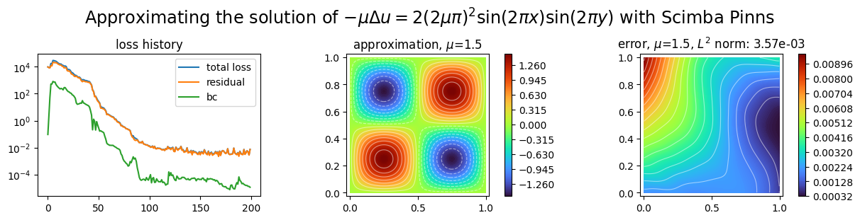
Plotting the approximation

import matplotlib.pyplot as plt
from scimba_torch.plots.plots_nd import plot_abstract_approx_spaces

plot_abstract_approx_spaces(
    pinn.space,  # the approximation space
    domain_x,  # the spatial domain
    domain_mu,  # the parameter's domain
    loss=pinn.losses,  # optional plot of the loss: the losses
    error=exact_sol,  # optional plot of the approximation error: the exact solution
    draw_contours=True,  # plotting isolevel lines
    n_drawn_contours=20,  # number of isolevel lines,
    title=(
        "Approximating the solution of "
        r"$- \mu\Delta u = 2(2\mu\pi)^2 \sin(2\pi x) \sin(2\pi y)$"
        " with Scimba Pinns"
    ),
)
plt.show()

Setting floating point arithmetic precision

Use regular torch instruction for this:

torch.set_default_dtype(torch.float32)

scimba_torch.print_torch_setting()

torch device: cuda:0
torch floating point format: torch.float32
cuda devices:        1
cuda current device: 0
cuda device name:    Tesla V100-PCIE-16GB

Now re-define the PINN and solve it.

def solve_with_pinn(epochs=200, layer_sizes=[64], n_collocation=1000, n_bc_collocation=1000, verbose=False):
    domain_x = Square2D([(0.0, 1), (0.0, 1)], is_main_domain=True)
    domain_mu = [(1.0, 2.0)]

    sampler = TensorizedSampler(
        [DomainSampler(domain_x), UniformParametricSampler(domain_mu)]
    )

    space = NNxSpace(1, 1, GenericMLP, domain_x, sampler, layer_sizes=layer_sizes)

    pde = Laplacian2DDirichletStrongForm(space, f=f_rhs, g=f_bc)

    pinn = NaturalGradientPinnsElliptic(pde, bc_type="weak")

    start = timeit.default_timer()
    pinn.solve(epochs=epochs, n_collocation=n_collocation, n_bc_collocation=n_bc_collocation, verbose=verbose)
    end = timeit.default_timer()

    print("loss after optimization: ", pinn.best_loss)
    print("approximation time: %f s"%(end-start))



solve_with_pinn()

loss after optimization:  6780.8095703125
approximation time: 13.823631 s

Natural gradient preconditionning is not well suited for simple precision arithmetic.

Setting device

torch.set_default_device("cpu")
torch.set_default_dtype(torch.float64)

scimba_torch.print_torch_setting()

torch device: cpu
torch floating point format: torch.float64
cuda devices:        1
cuda current device: 0
cuda device name:    Tesla V100-PCIE-16GB

Now re-define the PINN and solve it.

solve_with_pinn()

loss after optimization:  0.003241823796156317
approximation time: 76.899619 s