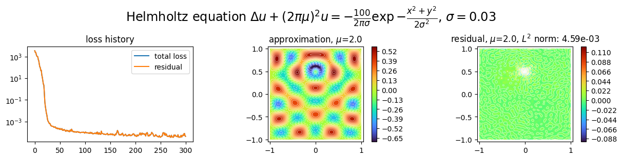
PINNs: Inhomogeneous Helmholtz equation

Solves the 2D inhomogeneous Helmholtz PDE with homogeneous Dirichlet BCs using a PINN.

\[\begin{split}\left\{\begin{array}{rl}\delta u + (2 \pi k)^2 u & = f \text{ in } \Omega \\ u & = 0 \text{ on } \partial \Omega\end{array}\right.\end{split}\]

where \(x = (x_1, x_2) \in \Omega = (-1, 1) \times (-1, 1)\), \(k = 2\) and \(f(x) = -\frac{100}{2\pi\sigma}\exp{\left(-\frac{x_1^2 + x_2^2}{2\sigma^2}\right)}\) with \(\sigma = 0.03\).

The boundary conditions are enforced strongly.

The neural network used is a simple MLP (Multilayer Perceptron) with multiscale Fourier features, and the optimization is done using Natural Gradient Descent.

from typing import Callable, Tuple

import matplotlib.pyplot as plt
import torch

from scimba_torch.approximation_space.abstract_space import AbstractApproxSpace
from scimba_torch.approximation_space.nn_space import NNxSpace
from scimba_torch.domain.meshless_domain.domain_2d import Square2D
from scimba_torch.integration.monte_carlo import DomainSampler, TensorizedSampler
from scimba_torch.integration.monte_carlo_parameters import UniformParametricSampler
from scimba_torch.neural_nets.coordinates_based_nets.features import (
    MultiScaleFourierMLP,
)
from scimba_torch.numerical_solvers.elliptic_pde.pinns import (
    NaturalGradientPinnsElliptic,
)
from scimba_torch.optimizers.optimizers_data import OptimizerData
from scimba_torch.plots.plots_nd import plot_abstract_approx_spaces
from scimba_torch.utils.scimba_tensors import LabelTensor, MultiLabelTensor
from scimba_torch.utils.typing_protocols import VarArgCallable

torch.manual_seed(0)


class HelmholtzDirichlet:
    def __init__(
        self,
        space: AbstractApproxSpace,
        spatial_dim: int,
        f: Callable,
        g: Callable,
        **kwargs,
    ):
        self.space = space
        self.spatial_dim = spatial_dim
        self.f = f
        self.g = g

        self.linear = True
        self.residual_size = 1
        self.bc_residual_size = 1

    def grad(
        self,
        w: torch.Tensor | MultiLabelTensor,
        y: torch.Tensor | LabelTensor,
    ) -> torch.Tensor | Tuple[torch.Tensor, ...]:
        return self.space.grad(w, y)

    def rhs(self, w: MultiLabelTensor, x: LabelTensor, mu: LabelTensor) -> torch.Tensor:
        return self.f(x, mu)

    def bc_rhs(
        self, w: MultiLabelTensor, x: LabelTensor, n: LabelTensor, mu: LabelTensor
    ) -> LabelTensor:
        return self.g(x, mu)

    def operator(
        self, w: MultiLabelTensor, x: LabelTensor, mu: LabelTensor
    ) -> torch.Tensor:
        u = w.get_components()
        k = mu.get_components()

        omega = 2.0 * torch.pi * k
        omega2_u = omega**2 * u

        grad_u = torch.cat(tuple(self.grad(u, x)), dim=-1)
        div_grad_u = tuple(self.grad(grad_u[:, 0], x))[0]
        for i in range(1, self.spatial_dim):
            div_grad_u += tuple(self.grad(grad_u[:, i], x))[i]

        return omega2_u + div_grad_u

    def functional_operator(
        self,
        func: VarArgCallable,
        x: torch.Tensor,
        mu: torch.Tensor,
        theta: torch.Tensor,
    ) -> torch.Tensor:
        omega = 2.0 * torch.pi * mu[0]
        omega2_u = omega**2 * func(x, mu, theta)

        grad_u = torch.func.jacrev(func, 0)
        grad_grad_u = torch.func.jacrev(grad_u, 0)(x, mu, theta).squeeze()
        div_grad_u = torch.einsum("ii", grad_grad_u)

        return omega2_u + div_grad_u

    # Dirichlet conditions
    def bc_operator(
        self, w: MultiLabelTensor, x: LabelTensor, n: LabelTensor, mu: LabelTensor
    ) -> torch.Tensor:
        u = w.get_components()
        return u

    def functional_operator_bc(
        self,
        func: VarArgCallable,
        x: torch.Tensor,
        n: torch.Tensor,
        mu: torch.Tensor,
        theta: torch.Tensor,
    ) -> torch.Tensor:
        return func(x, mu, theta)

sigma = 0.03
center = [0.0, 0.5]


def f_rhs(x: LabelTensor, mu: LabelTensor):
    x1, x2 = x.get_components()
    # mu1 = mu.get_components()
    return (
        -100
        * torch.exp(
            -((x1 - center[0]) ** 2 + (x2 - center[1]) ** 2) / (2.0 * sigma**2.0)
        )
        / ((2.0 * torch.pi) * sigma)
    )


def f_bc(x: LabelTensor, mu: LabelTensor):
    x1, _ = x.get_components()
    return x1 * 0.0

a = 1.0

def post_processing(inputs: torch.Tensor, x: LabelTensor, mu: LabelTensor):
    x1, x2 = x.get_components()
    return inputs * (-a - x1) * (a - x1) * (-a - x2) * (a - x2)


def functional_post_processing(func, x, mu, theta) -> torch.Tensor:
    return func(x, mu, theta) * (-a - x[0]) * (a - x[0]) * (-a - x[1]) * (a - x[1])

domain_mu = [(2.0, 2.0 + 1e-4)]
domain_x = Square2D([(-a, a), (-a, a)], is_main_domain=True)
sampler = TensorizedSampler(
    [DomainSampler(domain_x), UniformParametricSampler(domain_mu)]
)

space = NNxSpace(
    1,
    1,
    MultiScaleFourierMLP,
    domain_x,
    sampler,
    layer_sizes=[20, 20],
    means=[0.0, 0.0],
    stds=[4.0, 8.0],
    nb_features=20,
    activation_type="sine",
    post_processing=post_processing,
)

pde = HelmholtzDirichlet(space, 2, f=f_rhs, g=f_bc)
#
pinns = NaturalGradientPinnsElliptic(
    pde,
    bc_type="strong",
    functional_post_processing=functional_post_processing,
    matrix_regularization=2e-4,
)

pinns.solve(epochs=300, n_collocation=10000, verbose=False)

plot_abstract_approx_spaces(
    pinns.space,
    domain_x,
    domain_mu,
    loss=pinns.losses,
    residual=pinns.pde,
    draw_contours=True,
    n_drawn_contours=20,
    parameters_values="mean",
    title="Helmholtz equation $\\Delta u + (2\\pi\\mu)^2 u = -\\frac{100}{2\\pi\\sigma}\\exp{-\\frac{x^2 + y^2}{2\\sigma^2}}$, $\\sigma = 0.03$",
)

plt.show()