Using Time-Discrete Schemes

This tutorial covers the use of some time-discrete schemes available in Scimba for solving the rotating transport problem:

\[\begin{split}\left\{\begin{array}{lll} \partial_t u + a({\bf x}) \cdot \nabla u &= 0, & {\bf x}\in\Omega, t\in (0,1)\\ u(0,{\bf x},\mu) &= u_0({\bf x},\mu), & {\bf x}\in\Omega \\ u(t,{\bf x},\mu) &= 0, & {\bf x}\in\partial\Omega, t\in (0,1) \end{array}\right.\end{split}\]

where: \(\mu = (v,c)\), \({\bf x} = (x, y)\), \(\Omega\) is the unit disk and

\[\begin{split}a({\bf x}) := \left( \begin{array}{c} 2\pi y \\ -2\pi x \end{array}\right),\end{split}\]

with initial condition

\[u_0({\bf x},\mu) := u_{ex}(0,{\bf x},\mu)\]

where

\[u_{ex}(t,{\bf x},\mu) := 1 + \text{exp}\left( -\dfrac{1}{v^2} \left( \left( x - c \cos(2\pi t)\right)^2 + \left( y - c \sin(2\pi t)\right)^2 \right) \right).\]

is the exact solution of the considered problem.

Scimba implements discrete PINNS, Neural Galerkin and Neural Semi-Lagrangian time discrete schemes; let us first define a pde implementing the rotating transport.

Model definition

We first define a class named RotatingTransport to model our problem. This class inherits from the abstract class TemporalPDE.

from typing import Callable

import torch

from scimba_torch.approximation_space.abstract_space import AbstractApproxSpace
from scimba_torch.physical_models.temporal_pde.abstract_temporal_pde import TemporalPDE
from scimba_torch.utils.scimba_tensors import LabelTensor, MultiLabelTensor


class RotatingTransport(TemporalPDE):
    def __init__(self, space: AbstractApproxSpace, a: Callable, f_ic: Callable):
        self.space = space
        self.a = a
        self.f_ic = f_ic

    def grad(self, w: torch.Tensor, z: torch.Tensor) -> torch.Tensor:
        # returns the gradient of w with respect to z
        return self.space.grad(w, z)

    # the right hand side of the equation; w is the evaluation of the approximation at
    # t, x, y, mu
    def rhs(
        self, w: MultiLabelTensor, t: LabelTensor, xy: LabelTensor, mu: LabelTensor
    ) -> torch.Tensor:
        x, _ = xy.get_components()
        return 0 * x

    def bc_rhs(  # the left hand side of the boundary conditions
        self,
        w: MultiLabelTensor,
        t: LabelTensor,
        xy: LabelTensor,
        n: LabelTensor,
        mu: LabelTensor,
    ) -> torch.Tensor:
        x, _ = xy.get_components()
        return 0 * x

    def initial_condition(  # the left hand side of the initial conditions
        self, xy: LabelTensor, mu: LabelTensor
    ) -> torch.Tensor:
        return self.f_ic(xy, mu)

    def time_operator(  # the time dependant part of the left hand side of the equation
        self, w: MultiLabelTensor, t: LabelTensor, xy: LabelTensor, mu: LabelTensor
    ) -> torch.Tensor:
        return self.grad(w, t)

    # the space dependant part of the left hand side of the equation
    def space_operator(
        self, w: MultiLabelTensor, t: LabelTensor, xy: LabelTensor, mu: LabelTensor
    ) -> torch.Tensor:
        grad_u = torch.cat(list(self.grad(w.get_components(), xy)), dim=1)
        return torch.einsum("bi,bi-> b", self.a(t, xy, mu), grad_u)[..., None]

    def operator(  # already defined in TemporalPDE; given here for completeness
        self, w: MultiLabelTensor, t: LabelTensor, xy: LabelTensor, mu: LabelTensor
    ) -> torch.Tensor:
        return self.space_operator(w, t, xy, mu) + self.time_operator(w, t, xy, mu)

    # Dirichlet condition: u(t, x, mu) = 0
    def bc_operator(  # the left hand side of the equation
        self,
        w: MultiLabelTensor,
        t: LabelTensor,
        x: LabelTensor,
        n: LabelTensor,
        mu: LabelTensor,
    ) -> torch.Tensor:
        return w.get_components()

Now, we implement the exact solution, the initial condition and the advection vector field \(a\) with functions:

def exact_solution(t: LabelTensor, xy: LabelTensor, mu: LabelTensor) -> torch.Tensor:
    x, y = xy.get_components()
    t_ = t.get_components()
    c, v = mu.get_components()
    x_t = torch.cos(2 * torch.pi * t_)
    y_t = torch.sin(2 * torch.pi * t_)
    return 1 + torch.exp(-0.5 / v**2 * ((x - c * x_t) ** 2 + (y - c * y_t) ** 2))


def initial_condition(xy: LabelTensor, mu: LabelTensor) -> torch.Tensor:
    t = LabelTensor(torch.zeros((xy.shape[0], 1)))
    return exact_solution(t, xy, mu)


def a(t: LabelTensor, xy: LabelTensor, mu: LabelTensor) -> torch.Tensor:
    x, y = xy.get_components()
    return torch.cat((-2 * torch.pi * y, 2 * torch.pi * x), dim=1)

We also define a geometric domain modeling \(\Omega\), a sampler on \(\Omega\) and specialize our problem to \(\mu = (0.3, 0.1)\).

from scimba_torch.domain.meshless_domain.domain_2d import Disk2D
from scimba_torch.integration.monte_carlo import DomainSampler, TensorizedSampler
from scimba_torch.integration.monte_carlo_parameters import UniformParametricSampler

torch.random.manual_seed(0)

domain_x = Disk2D((0.0, 0.0), 1.0, is_main_domain=True)
domain_mu = [[0.3, 0.3], [0.1, 0.1]]

sampler = TensorizedSampler(
    [
        DomainSampler(domain_x),
        UniformParametricSampler(domain_mu),
    ]
)

Solving the rotating transport problem with a discrete PINN

We first define a projection space to compute the numerical approximation as a generic MLP with 3 hidden layers of respective sizes 8, 16 and 8, and create a pde:

from scimba_torch.approximation_space.nn_space import NNxSpace
from scimba_torch.neural_nets.coordinates_based_nets.mlp import GenericMLP

space0 = NNxSpace(1, 2, GenericMLP, domain_x, sampler, layer_sizes=[8, 16, 8])
pde0 = RotatingTransport(space0, a, initial_condition)

One must now define a projector to compute approximation at each time step; here we use a projector using a natural gradient descent algorithms, namely Energy Natural Gradient:

from scimba_torch.numerical_solvers.temporal_pde.time_discrete import (
    TimeDiscreteNaturalGradientProjector,
)

projector0 = TimeDiscreteNaturalGradientProjector(pde0)

One can now define a discrete PINN for the rotating transport problem as follows:

from scimba_torch.numerical_solvers.temporal_pde.discrete_pinn import DiscretePINN

scheme0 = DiscretePINN(pde0, projector0, scheme="rk4")

Here we use 4-th order Runge-Kutta time integration scheme; other scheme available are explicit Euler ("euler_exp") and 2-th order Runge-Kutta ("rk2").

The first step is to project the initial solution onto the approximation space:

scheme0.initialization(epochs=200, n_collocation=15_000, verbose=False)

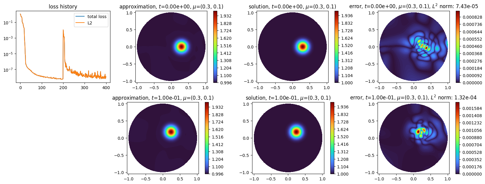
We choose time-steps of \(0.02\) to get an approximation of a solution for \(t = 0.1\):

scheme0.solve(dt=0.02, T=0.1, epochs=20, n_collocation=15_000, verbose=False)

and plot the approximated solution, the exact solution and the error absolute:

import matplotlib.pyplot as plt

from scimba_torch.plots.plot_time_discrete_scheme import plot_time_discrete_scheme

plot_time_discrete_scheme(
    scheme0,
    solution=exact_solution,
    error=exact_solution,
)

plt.show()

by default, the space approximating the initial condition and the solution for one intermediate time is saved and displayed; this can be adjusted by using optional argument nb_keep of the solve method as demonstrated below.

Solving the rotating transport problem with the Neural Galerkin approach

We create an approximation space, a pde object and a projector as previously:

from scimba_torch.approximation_space.nn_space import NNxSpace
from scimba_torch.neural_nets.coordinates_based_nets.mlp import GenericMLP
from scimba_torch.numerical_solvers.temporal_pde.time_discrete import (
    TimeDiscreteNaturalGradientProjector,
)

space1 = NNxSpace(1, 2, GenericMLP, domain_x, sampler, layer_sizes=[8, 16, 8])
pde1 = RotatingTransport(space1, a, initial_condition)
projector1 = TimeDiscreteNaturalGradientProjector(pde1)

then the Neural Galerkin solver with 4-th order Runge-Kutta time integrator is defined and initialized with

from scimba_torch.numerical_solvers.temporal_pde.neural_galerkin import NeuralGalerkin

scheme1 = NeuralGalerkin(pde1, projector1, scheme="rk4")
scheme1.initialization(epochs=200, n_collocation=15_000, verbose=False)

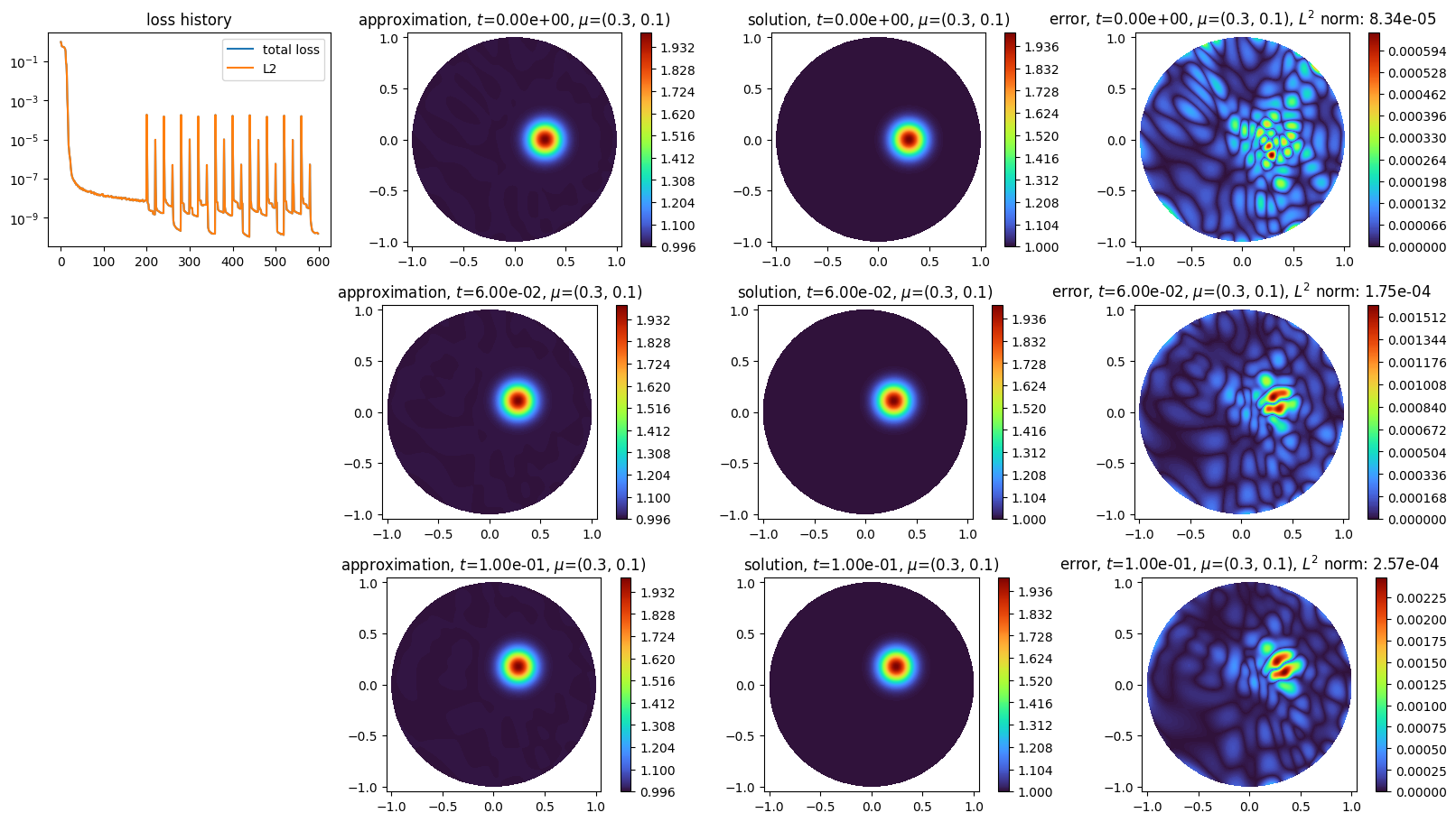
We choose time-steps of \(0.02\) to get an approximation of a solution for \(t = 0.5\):

scheme1.solve(dt=0.02, T=0.5, verbose=False, nb_keep=2)

import matplotlib.pyplot as plt

from scimba_torch.plots.plot_time_discrete_scheme import plot_time_discrete_scheme

plot_time_discrete_scheme(
    scheme1,
    solution=exact_solution,
    error=exact_solution,
)

plt.show()

Notice the use of the optional argument nb_keep in the solve method to keep more than one intermediate approximated solution.

Solving the rotating transport problem with the Neural Semi-Lagrangian approach

As Neural Semi-Lagrangian approach is defined for advection diffusion problems, the class modeling the problem needs a flag specifying wether the advection is constant or not:

class RotatingTransport(RotatingTransport):
    def __init__(self, space: AbstractApproxSpace, a: Callable, f_ic: Callable):
        super().__init__(space, a, f_ic)
        self.constant_advection = False

We create an approximation space, a pde object and a projector as previously:

from scimba_torch.approximation_space.nn_space import NNxSpace
from scimba_torch.neural_nets.coordinates_based_nets.mlp import GenericMLP
from scimba_torch.numerical_solvers.temporal_pde.time_discrete import (
    TimeDiscreteNaturalGradientProjector,
)

space2 = NNxSpace(1, 2, GenericMLP, domain_x, sampler, layer_sizes=[8, 16, 8])
pde2 = RotatingTransport(space2, a, initial_condition)
projector2 = TimeDiscreteNaturalGradientProjector(pde2)

In order to apply semi-lagrangian, one needs first to generate the characteristic curves, which is done in Scimba with the class Characteristic:

from scimba_torch.numerical_solvers.temporal_pde.neural_semilagrangian import (
    Characteristic,
    NeuralSemiLagrangian,
)

characteristic = Characteristic(pde2)

One can now define a neural semi-lagrangian solver with this characteristic and initialize it:

scheme2 = NeuralSemiLagrangian(characteristic, projector2)
scheme2.initialization(epochs=200, n_collocation=15_000, verbose=False)

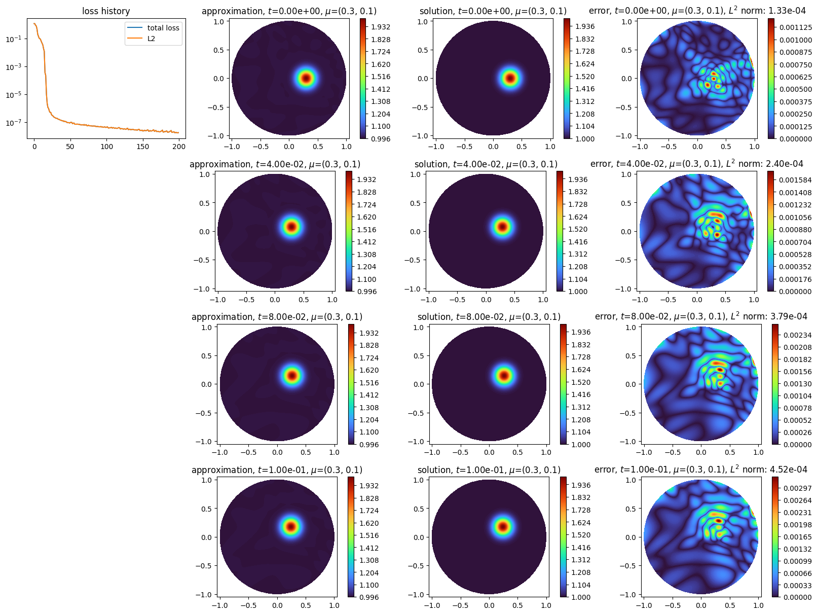
With neural semi-lagrangian, one can use much wider time steps than with previous methods:

scheme2.solve(dt=0.25, T=0.5, epochs=200, verbose=False)

import matplotlib.pyplot as plt

from scimba_torch.plots.plot_time_discrete_scheme import plot_time_discrete_scheme

plot_time_discrete_scheme(
    scheme2,
    solution=exact_solution,
    error=exact_solution,
)

plt.show()

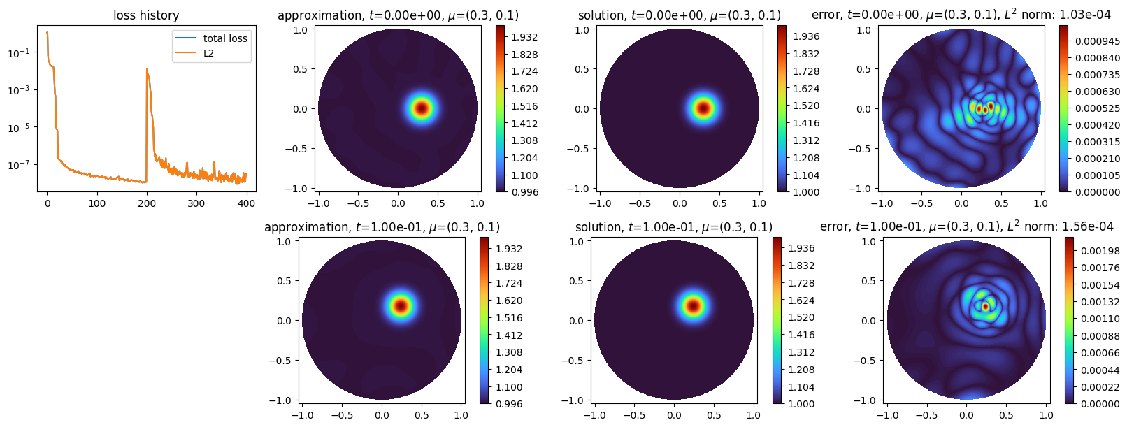
We finally show how to use an exactly defined characteristic curve in the neural semi-lagrangian solver; in the rotating transport example it is:

def exact_foot(
    t: torch.Tensor, xy: LabelTensor, mu: LabelTensor, dt: float
) -> torch.Tensor:
    x, y = xy.get_components()

    arg = 2 * torch.pi * t
    c_n = torch.cos(arg)
    s_n = torch.sin(arg)

    k1 = x * s_n + y * c_n
    k2 = x * c_n - y * s_n

    arg_np1 = 2 * torch.pi * (t + dt)
    c_np1 = torch.cos(arg_np1)
    s_np1 = torch.sin(arg_np1)

    x_np1 = k1 * s_np1 + k2 * c_np1
    y_np1 = -k2 * s_np1 + k1 * c_np1

    return torch.cat((x_np1, y_np1), dim=1)

One can now create the Characteristic object with this exact definition, and apply the solver as previously:

space3 = NNxSpace(1, 2, GenericMLP, domain_x, sampler, layer_sizes=[8, 16, 8])
pde3 = RotatingTransport(space3, a, initial_condition)
projector3 = TimeDiscreteNaturalGradientProjector(pde3)
# use the exact definition of the characteristic curve:
characteristic = Characteristic(pde3, exact_foot=exact_foot)

scheme3 = NeuralSemiLagrangian(characteristic, projector3)
scheme3.initialization(epochs=200, n_collocation=15_000, verbose=False)

scheme3.solve(dt=0.25, T=0.5, epochs=200, verbose=False)

import matplotlib.pyplot as plt

from scimba_torch.plots.plot_time_discrete_scheme import plot_time_discrete_scheme

plot_time_discrete_scheme(
    scheme3,
    solution=exact_solution,
    error=exact_solution,
)

plt.show()