Defining a physical model
This tutorial will present the main steps to implement the modelisation of a physical problem involving Partial Differential Equation (PDE) in Scimba, for 4 kinds of problems:
1-dimensional unknown function of space in homogeneous medium
1-dimensional unknown function of time and space in homogeneous medium
2-dimensional unknown function of time and space in homogeneous medium
1-dimensional unknown function of space in non-homogeneous medium
[1]:
import matplotlib.pyplot as plt
import torch
1-dimensional unknown function of space in homogeneous medium
In this first section, we will implement a 2D Laplacian with Dirichlet boundary conditions in an homogenous medium.
We consider the equation:
on \((x,y) \in \Omega := [0, 1]\times[0, 1]\) with parameter \(\mu\in[1,2]\) subject to the Dirichlet condition:
on \(\partial\Omega\).
The strong form of this problem will be implemented as a class, and an instance of this class will serve numerical approximation of the solution with a PINN.
Remark: the strong form of this problem is already implemented in the class Laplacian2DDirichletStrongForm and can be directly used by users with:
[2]:
from scimba_torch.physical_models.elliptic_pde.laplacians import (
    Laplacian2DDirichletStrongForm,
)

try:
    pde = Laplacian2DDirichletStrongForm(space, f=f_rhs, g=f_bc)  # noqa: F821
except Exception:
    pass
where space is an approximation space and f_rhs and f_bc are the right hand sides of the equation and the boundary condition; see the complete example about Scimba basics.
The rest of this section describes the implementation of this class in a pedagogical aim.
Instead of implementing the class from scratch, and as our problem is an elliptic one, we will define it as a subclass of StrongFormEllipticPDE, itself a subclass of:
[3]:
from abc import ABC

from scimba_torch.approximation_space.abstract_space import AbstractApproxSpace


class EllipticPDE(ABC):
    def __init__(self, space: AbstractApproxSpace, linear: bool = False, **kwargs):
        super().__init__()
        self.space = space  # a parameterized function to approximate the unknown
        # whether the left hand side of the equation is linear in the unknown's
        # derivatives
        self.linear = linear

    def grad(
        self,
        # the evaluation of self.space at a batched tensor of spatial points
        w: torch.Tensor,
        z: torch.Tensor,  # a tensor
    ) -> torch.Tensor | tuple[torch.Tensor]:
        # returns the gradient of w with respect to z
        return self.space.grad(w, z)
here comes the definition of the abstract class StrongFormEllipticPDE of which we will define a subclass:
[4]:
from abc import abstractmethod

from scimba_torch.utils.scimba_tensors import LabelTensor, MultiLabelTensor


class StrongFormEllipticPDE(EllipticPDE):
    def __init__(
        self,
        space: AbstractApproxSpace,  # see above
        linear: bool = False,  # see above
        residual_size: int = 1,  # the number of scalar equations inside the domain
        # the number of scalar equations for the boundary conditions
        bc_residual_size: int = 0,
        **kwargs,
    ):
        super().__init__(space, linear, **kwargs)
        self.residual_size = residual_size
        self.bc_residual_size = bc_residual_size

    @abstractmethod
    def rhs(
        self, w: MultiLabelTensor, xy: LabelTensor, mu: LabelTensor
    ) -> torch.Tensor:
        """the right hand side of the equation; w is the evaluation of the approximation
        at x, y, mu"""
        pass

    @abstractmethod
    def operator(
        self, w: MultiLabelTensor, xy: LabelTensor, mu: LabelTensor
    ) -> torch.Tensor:
        """the left hand side of the equation"""
        pass

    @abstractmethod
    def bc_rhs(
        self, w: MultiLabelTensor, xy: LabelTensor, n: LabelTensor, mu: LabelTensor
    ) -> torch.Tensor:
        """the left hand side of the boundary conditions"""
        pass

    @abstractmethod
    def bc_operator(
        self, w: MultiLabelTensor, xy: LabelTensor, n: LabelTensor, mu: LabelTensor
    ) -> torch.Tensor:
        """the right hand side of the boundary conditions"""
        pass
Notice that both left and right hand sides of boundary condition equation definition also take as argument a n:labelTensor which contains the normals at xy values.
Let us now implement our problem in the class Laplacian2DDirichlet:
[5]:
from typing import Callable

from scimba_torch.approximation_space.abstract_space import AbstractApproxSpace
from scimba_torch.utils.scimba_tensors import LabelTensor, MultiLabelTensor
from scimba_torch.utils.typing_protocols import VarArgCallable


class Laplacian2DDirichlet(StrongFormEllipticPDE):
    def __init__(self, space: AbstractApproxSpace, f: Callable, g: Callable, **kwargs):
        super().__init__(
            space, linear=True, residual_size=1, bc_residual_size=1, **kwargs
        )
        self.f = f
        self.g = g

    def rhs(self, w, xy, mu):  # the right hand side of the equation
        return self.f(xy, mu)

    def bc_rhs(self, w, xy, n, mu):  # the left hand side of the equation
        return self.g(xy, mu)

    def operator(self, w, xy, mu):
        u = (
            w.get_components()
        )  # the values of the approximation u evaluated at x, y, mu
        alpha = mu.get_components()  # the mu values
        u_x, u_y = self.grad(
            u, xy
        )  # the first order derivatives of u with respect to x and y
        u_xx, _ = self.grad(u_x, xy)  # the second order derivative with respect to x, x
        _, u_yy = self.grad(u_y, xy)  # the second order derivative with respect to y, y
        return -alpha * (
            u_xx + u_yy
        )  # the left hand side of the equation inside the domain

    # Dirichlet condition: u(x,y,mu) = 0
    def bc_operator(self, w, xy, n, mu):
        u = (
            w.get_components()
        )  # the values of the approximation u evaluated at x, y, mu
        return u  # the left hand side of the boundary condition
This is enough if one wants to compute an approximation with a PINN using classical ADAM, gradient descent or LBFGS optimization algorithm to minimize the residue.
In order to use natural gradient descent algorithms one needs to work a bit more. Such approaches require to combine differentiation with respect to the physical variables of the problem and with respect to the parameters of the approximation space in use, which is a Neural Network implemented with a torch.nn.module.
In order to do so, Scimba requires implementations of the left hand sides of:
the operator,
and the boundary condition
as functions that can be vmapped with torch.func.vmap.
These functions must be called respectively:
functional_operatorfunctional_operator_bc
Below are examples of such implementation for the operator and boundary condition above:
[6]:
class Laplacian2DDirichlet(Laplacian2DDirichlet):
    def functional_operator(
        self,
        u: VarArgCallable,  # the approximation u
        # u(xy, mu, theta) is a (1,) shaped tensor
        xy: torch.Tensor,  # xy as a torch tensor of shape (2,)
        mu: torch.Tensor,  # mu as a torch tensor of shape (1,)
        theta: torch.Tensor,  # the parameters theta of the approximation space
    ) -> torch.Tensor:
        # compute the map
        # u'(xy, mu, theta) := ( du/dx(xy, mu, theta), du/dy(xy, mu, theta) )
        map_grad_u = torch.func.jacrev(
            u, 0
        )  # 0 is the index of xy in the variables list of u
        # compute the map
        # u''(xy, mu, theta) := ( d2u/dxdx(xy, mu, theta), d2u/dxdy(xy, mu, theta)
        #                         d2u/dxdy(xy, mu, theta), d2u/dydy(xy, mu, theta) )
        map_hessian_u = torch.func.jacrev(
            map_grad_u, 0
        )  # 0 is the index of xy in the variables list of u
        # evaluate it
        hessian_u = map_hessian_u(xy, mu, theta).squeeze()  # shape (2,2,)
        # compute the right hand side of the equation
        return -mu * (hessian_u[0, 0] + hessian_u[1, 1])  # shape (1,)
where the argument u is a functional version of the approximation function, depending on xy, mu and the parameters theta such as:
[7]:
def u(xy: torch.Tensor, mu: torch.Tensor, theta: torch.Tensor) -> torch.Tensor: ...
that returns the evaluation of the numerical approximation u at non-batched value (xy,mu) for parameters theta. The latter has not to be implemented, it is crafted by Scimba. It output a torch tensor of shape (m,) where m is the output dimension of u; here 1.
When writting the functional_operator, it is important to keep in mind that it will be vmapped for all the variables except theta. As a consequence, it is implemented as a function taking in input non-batched physical variables; for instance here, input xy has shape (2,) as \(\Omega\) has dimension 2.
It has to return a torch tensor of shape (m,) where m is the number of equations of the residual, here 1.
It will be transformed in a batched function during the torch vectorialization process.
In the body of the function, derivatives with respect of the physical variables \(\dfrac{\partial}{\partial x}u\) or \(\dfrac{\partial}{\partial y}u\) are obtained by applying the differentiation functional operator torch.func.jacrev(...) to u or its derivatives.
the functional operator for the boundary condition is:
[8]:
class Laplacian2DDirichlet(Laplacian2DDirichlet):
    def functional_operator_bc(
        self,
        u: VarArgCallable,
        x: torch.Tensor,
        n: torch.Tensor,
        mu: torch.Tensor,
        theta: torch.Tensor,
    ) -> torch.Tensor:
        return u(x, mu, theta)
We finish this subsection by using a PINN and Energy Natural Gradient Descent to compute an approximation of the solution:
[9]:
from scimba_torch.approximation_space.nn_space import NNxSpace
from scimba_torch.domain.meshless_domain.domain_2d import Square2D
from scimba_torch.integration.monte_carlo import DomainSampler, TensorizedSampler
from scimba_torch.integration.monte_carlo_parameters import UniformParametricSampler
from scimba_torch.neural_nets.coordinates_based_nets.mlp import GenericMLP
from scimba_torch.numerical_solvers.elliptic_pde.pinns import (
NaturalGradientPinnsElliptic,
)
from scimba_torch.plots.plots_nd import plot_abstract_approx_spaces
# \Omega and parameter's domain
domain_x = Square2D([(0.0, 1), (0.0, 1)], is_main_domain=True)
domain_mu = [(1.0, 2.0)]
# a sampler on \Omega\times[1,2]
sampler = TensorizedSampler(
[DomainSampler(domain_x), UniformParametricSampler(domain_mu)]
)
# the right hand side of the residual
def f_rhs(xs: LabelTensor, ms: LabelTensor) -> torch.Tensor:
x, y = xs.get_components()
mu = ms.get_components()
pi = torch.pi
return 2 * (2.0 * mu * pi) ** 2 * torch.sin(2.0 * pi * x) * torch.sin(2.0 * pi * y)
# the right hand side of the boundary condition
def f_bc(xs: LabelTensor, ms: LabelTensor) -> torch.Tensor:
x, _ = xs.get_components()
return x * 0.0
# a space of parameterized functions u_\theta to approximate u
space = NNxSpace(
1, # the output dimension of u_\theta
1, # the parameter's space dimension
GenericMLP, # the type of neural network
domain_x, # the geometric domain
sampler, # the sampler
layer_sizes=[64], # the size of intermediate layers of the nn
)
pde = Laplacian2DDirichlet(space, f=f_rhs, g=f_bc)
pinns = NaturalGradientPinnsElliptic(pde, bc_type="weak")
pinns.solve(epochs=200, n_collocation=1000, n_bc_collocation=1000)
# the solution
def exact_sol(xs: LabelTensor, ms: LabelTensor) -> torch.Tensor:
x, y = xs.get_components()
mu = ms.get_components()
pi = torch.pi
return mu * torch.sin(2.0 * pi * x) * torch.sin(2.0 * pi * y)
plot_abstract_approx_spaces(
pinns.space, # the approximation space
domain_x, # the spatial domain
domain_mu, # the parameter's domain
loss=pinns.losses, # optional plot of the loss: the losses
error=exact_sol, # optional plot of the approximation error: the exact solution
draw_contours=True, # plotting isolevel lines
n_drawn_contours=20, # number of isolevel lines,
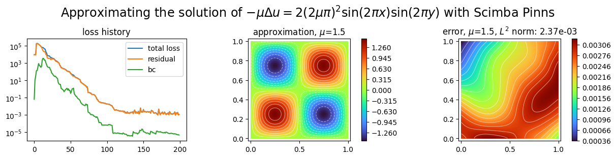
title=(
"Approximating the solution of "
r"$- \mu\Delta u = 2(2\mu\pi)^2 \sin(2\pi x) \sin(2\pi y)$"
" with Scimba Pinns"
),
)
plt.show()
Scimba_jax uses device: [CpuDevice(id=0)]
Scimba_jax uses dtype: <class 'jax.numpy.float64'>
Training: 100%|||||||||||||||||| 200/200[00:04<00:00] , loss: 1.0e+04 -> 1.3e-02
1-dimensional unknown function of time and space in homogeneous medium
We consider a time-dependant 1D heat equation in an homogenous medium:
on \(x \in \Omega := [0, 1]\) with parameter \(\mu\in[0, 1]\) subject to the Dirichlet condition:
on \(\partial\Omega\), and the initial condition:
The strong form of this problem will be implemented as a class of which an instance will be used for solving with a PINN.
Remark: the strong form of this problem is already implemented in the class HeatEquation1DDirichletStrongForm, and the following deserves a pedagogical aim.
We describe two ways of implementing the considered problem:
as a spatio-temporal model,
as a temporal extension of a spatial model (a 1D laplacian).
Implementation as a spatio-temporal problem
This time, we will implement a class modeling this problem from scratch.
[10]:
from typing import Callable

from scimba_torch.approximation_space.abstract_space import AbstractApproxSpace
from scimba_torch.utils.scimba_tensors import LabelTensor, MultiLabelTensor
from scimba_torch.utils.typing_protocols import VarArgCallable


class Heat1DDirichlet:
    def __init__(
        self, space: AbstractApproxSpace, f_ic: Callable, f: Callable, f_bc: Callable
    ):
        self.space = space
        self.f_ic = f_ic
        self.f = f
        self.f_bc = f_bc
        self.linear = True
        self.residual_size = 1
        self.bc_residual_size = 1
        self.ic_residual_size = 1

    def grad(self, w: torch.Tensor, y: torch.Tensor) -> torch.Tensor:
        # returns the gradient of w with respect to z
        return self.space.grad(w, y)

    def rhs(
        self, w: MultiLabelTensor, t: LabelTensor, x: LabelTensor, mu: LabelTensor
    ) -> torch.Tensor:
        """the right hand side of the equation; w is the evaluation of the approximation
        at x, y, mu"""
        return self.f(t, x, mu)

    def bc_rhs(  # the left hand side of the boundary conditions
        self,
        w: MultiLabelTensor,
        t: LabelTensor,
        x: LabelTensor,
        n: LabelTensor,
        mu: LabelTensor,
    ) -> torch.Tensor:
        return self.f_bc(t, x, mu)

    def init(  # the left hand side of the boundary conditions
        self, x: LabelTensor, mu: LabelTensor
    ) -> torch.Tensor:
        return self.f_ic(x, mu)

    def space_operator(
        self, w: MultiLabelTensor, t: LabelTensor, x: LabelTensor, mu: LabelTensor
    ) -> torch.Tensor:
        """the space dependant part of the left hand side of the equation"""
        u = w.get_components()
        alpha = mu.get_components()
        u_xx = self.grad(self.grad(u, x), x)
        return -alpha * u_xx

    def time_operator(  # the time dependant part of the left hand side of the equation
        self, w: MultiLabelTensor, t: LabelTensor, x: LabelTensor, mu: LabelTensor
    ) -> torch.Tensor:
        u = w.get_components()
        dudt = self.grad(u, t)
        return dudt

    def operator(  # the left hand side of the equation
        self, w: MultiLabelTensor, t: LabelTensor, x: LabelTensor, mu: LabelTensor
    ) -> torch.Tensor:
        return self.space_operator(w, t, x, mu) + self.time_operator(w, t, x, mu)

    # Dirichlet condition: u(t, x, mu) = 0
    def bc_operator(  # the left hand side of the equation
        self,
        w: MultiLabelTensor,
        t: LabelTensor,
        x: LabelTensor,
        n: LabelTensor,
        mu: LabelTensor,
    ) -> torch.Tensor:
        u = w.get_components()
        return u
As previously, using natural gradient descent algorithms requires to include to the definition of the class implementations of
the operator
the boundary condition operator
the initial condition operator
as functions that can be vmapped with torch.func.vmap.
These functions must be called respectively:
functional_operatorfunctional_operator_bcfunctional_operator_ic
[11]:
class Heat1DDirichlet(Heat1DDirichlet):
    def functional_operator(
        self,
        u: VarArgCallable,
        t: torch.Tensor,
        x: torch.Tensor,
        mu: torch.Tensor,
        theta: torch.Tensor,
    ) -> torch.Tensor:
        # space operator
        hess_u = torch.func.jacrev(
            torch.func.jacrev(u, 1), 1
        )  # 1 is the index of x in the variables list
        space_op = -mu * hess_u(t, x, mu, theta).squeeze()
        # time operator
        time_op = torch.func.jacrev(u, 0)(
            t, x, mu, theta
        ).squeeze()  # 0 is the index of t in the variables list
        return time_op + space_op

    # Dirichlet conditions
    def functional_operator_bc(
        self,
        u: VarArgCallable,
        t: torch.Tensor,
        x: torch.Tensor,
        n: torch.Tensor,
        mu: torch.Tensor,
        theta: torch.Tensor,
    ) -> torch.Tensor:
        return u(t, x, mu, theta)

    def functional_operator_ic(
        self,
        u: VarArgCallable,
        x: torch.Tensor,
        mu: torch.Tensor,
        theta: torch.Tensor,
    ) -> torch.Tensor:
        t = torch.zeros_like(x)
        return u(t, x, mu, theta)
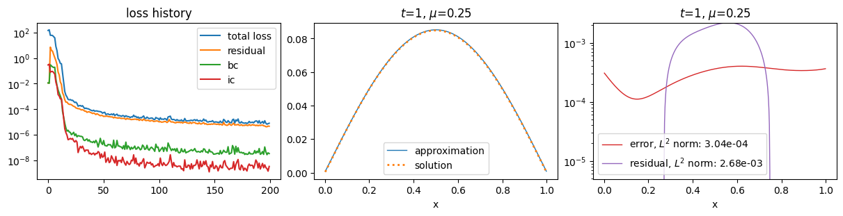
We finish this subsection by using a PINN and Energy Natural Gradient Descent to compute an approximation of the solution:
[12]:
from scimba_torch.approximation_space.nn_space import NNxtSpace
from scimba_torch.domain.meshless_domain.domain_1d import Segment1D
from scimba_torch.integration.monte_carlo import DomainSampler, TensorizedSampler
from scimba_torch.integration.monte_carlo_parameters import UniformParametricSampler
from scimba_torch.integration.monte_carlo_time import UniformTimeSampler
from scimba_torch.neural_nets.coordinates_based_nets.mlp import GenericMLP
from scimba_torch.numerical_solvers.temporal_pde.pinns import (
    NaturalGradientTemporalPinns,
)


def exact(t, x, mu):
    x1 = x.get_components()
    t1 = t.get_components()
    return torch.exp(-(t1 * torch.pi**2) / 4.0) * torch.sin(torch.pi * x1)


def f_rhs(t, x, mu):
    mu1 = mu.get_components()
    return 0 * mu1


def f_bc(t, x, mu):
    x1 = x.get_components()
    return 0 * x1


def f_ini(x, mu):
    t = LabelTensor(torch.zeros_like(x.x))
    return exact(t, x, mu)


domain_x = Segment1D((0, 1), is_main_domain=True)
t_min, t_max = 0.0, 1.0
domain_t = (t_min, t_max)
domain_mu = [(0.0, 0.5)]

sampler = TensorizedSampler(
    [
        UniformTimeSampler(domain_t),
        DomainSampler(domain_x),
        UniformParametricSampler(domain_mu),
    ]
)

space = NNxtSpace(1, 1, GenericMLP, domain_x, sampler, layer_sizes=[32, 32])
pde = Heat1DDirichlet(space, f_ic=f_ini, f=f_rhs, f_bc=f_bc)
pinn = NaturalGradientTemporalPinns(
    pde,
    bc_type="weak",
    ic_type="weak",
    bc_weight=50.0,
    ic_weight=500.0,
    matrix_regularization=1e-6,
)

pinn.solve(
    epochs=200,
    n_collocation=4000,
    n_bc_collocation=200,
    n_ic_collocation=100,
)

plot_abstract_approx_spaces(
    pinn.space,
    domain_x,
    domain_mu,
    domain_t,
    parameters_values=[0.25],
    time_values=[t_max],
    loss=pinn.losses,
    residual=pde,
    solution=exact,
    error=exact,
)

plt.show()
Training: 100%|||||||||||||||||| 200/200[00:29<00:00] , loss: 2.8e+02 -> 1.1e-05
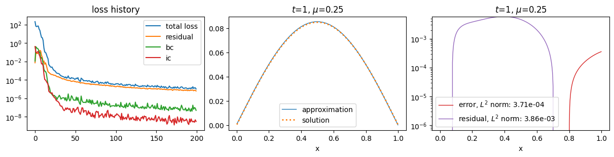
Implementation as a temporal extension of a 1D Laplacian
As for many time-dependent PDEs, the left-hand side of the heat equation:
is the sum of the first order time derivative of the unknown \(U\) and the left-hand side of a stationary PDE, here a 1D laplacian. Moreover the boundary condition is a classical Dirichlet condition.
This type of problem can be implemented in ScimBa in two steps:
first implement the stationary problem
second implement the time-depêndent problem as a class inheriting from the abstract class
GenericFirstOrderTemporalPDE.
Here the stationary is a 1D laplacian with Dirichlet boundary condition which is already implemented in ScimBa.
[13]:
from scimba_torch.physical_models.elliptic_pde.laplacians import (
    Laplacian1DDirichletStrongForm,
)
from scimba_torch.physical_models.temporal_pde.abstract_temporal_pde import (
    GenericFirstOrderTemporalPDE,
)

class Heat1DDirichletBis(GenericFirstOrderTemporalPDE):

    def __init__(
        self,
        space: AbstractApproxSpace,
        init: Callable,
        f: Callable | None = None,
        g: Callable | None = None,
        **kwargs,
    ):
        # Below we initialize rhs and bc_rhs of the
        # space component to default values because it will not be used;
        # rhs and bc_rhs of the time-dependent PDE are used instead
        space_component = Laplacian1DNeumannStrongForm(space)
        super().__init__(space, space_component, init, f, g, **kwargs)
Notice that the right-hand sides of the residuals of the spatial component are not used and thus are initialized to default values. Indead time-dependent right-hand sides might be used.
We finally define and train a PINN for this model:
[14]:
space = NNxtSpace(1, 1, GenericMLP, domain_x, sampler, layer_sizes=[32, 32])
pde = Heat1DDirichlet(space, f_ic=f_ini, f=f_rhs, f_bc=f_bc)
pinn = NaturalGradientTemporalPinns(
    pde,
    bc_type="weak",
    ic_type="weak",
    bc_weight=50.0,
    ic_weight=500.0,
    matrix_regularization=1e-6,
)

pinn.solve(
    epochs=200,
    n_collocation=4000,
    n_bc_collocation=200,
    n_ic_collocation=100,
)

plot_abstract_approx_spaces(
    pinn.space,
    domain_x,
    domain_mu,
    domain_t,
    parameters_values=[0.25],
    time_values=[t_max],
    loss=pinn.losses,
    residual=pde,
    solution=exact,
    error=exact,
)

plt.show()
Training: 100%|||||||||||||||||| 200/200[00:29<00:00] , loss: 2.1e+02 -> 1.0e-05
2-dimensional unknown function of time and space in homogeneous medium
We consider a time-dependant 1D problem with 2-dimentional unknown function \(u_1, u_2\):
on \(x \in \Omega := [0, 1]\) subject to the Dirichlet condition:
on \(\partial\Omega\), and the initial condition:
where \(D = 0.02\).
Since residual and boundary and initial conditions are systems of 2 equations of an unknown function \(u: \mathbb{R}\times\mathbb{R} \rightarrow \mathbb{R}^2\), left and right hand sides of the former will be functions returning tuples of torch tensors.
[15]:
from typing import Callable, Tuple

from scimba_torch.approximation_space.abstract_space import AbstractApproxSpace
from scimba_torch.utils.scimba_tensors import LabelTensor


class LinearizedEuler:
    def __init__(
        self,
        space: AbstractApproxSpace,
        init: Callable,
        f: Callable,
        g: Callable,
        **kwargs,
    ):
        self.space = space
        self.init = init
        self.f = f
        self.g = g

        self.linear = True
        self.residual_size = 2  # the number of equations of the residual
        self.bc_residual_size = 2  # the number of equations of the boundary condition
        self.ic_residual_size = 2  # the number of equations of the initial condition

    def grad(self, w, y):
        return self.space.grad(w, y)

    def rhs(self, w, t, x, mu) -> Tuple[torch.Tensor]:
        return self.f(t, x, mu)  # assume f returns a tuple of 2 tensors

    def bc_rhs(self, w, t, x, n, mu) -> Tuple[torch.Tensor]:
        return self.g(t, x, mu)  # assume g returns a tuple of 2 tensors

    def initial_condition(self, x, mu) -> Tuple[torch.Tensor]:
        return self.init(x, mu)  # assume init returns a tuple of 2 tensors

    def time_operator(self, w, t, x, mu) -> Tuple[torch.Tensor]:
        u, v = w.get_components()
        u_t = self.grad(u, t)
        v_t = self.grad(v, t)
        return u_t, v_t  # returns a tuple of 2 tensors

    def space_operator(self, w, t, x, mu) -> Tuple[torch.Tensor]:
        u, v = w.get_components()
        u_x = self.grad(u, x)
        v_x = self.grad(v, x)
        return v_x, u_x  # returns a tuple of 2 tensors

    def operator(self, w, t, x, mu) -> Tuple[torch.Tensor]:
        time_0, time_1 = self.time_operator(w, t, x, mu)
        space_0, space_1 = self.space_operator(w, t, x, mu)
        return time_0 + space_0, time_1 + space_1  # returns a tuple of 2 tensors

    # Dirichlet conditions
    def bc_operator(self, w, t, x, n, mu: LabelTensor) -> Tuple[torch.Tensor]:
        u, v = w.get_components()
        return u, v
As previously, one need to implement the functions
functional_operator,functional_operator_bc,and
functional_operator_ic.
They will not return tuples of torch tensors but tensors of shapes (2,); once vmapped, the returned tensors will have shapes (batch, 2).
[16]:
class LinearizedEuler(LinearizedEuler):
    def functional_operator(self, u, t, x, mu, theta) -> torch.Tensor:
        # space operator
        u_space = torch.func.jacrev(u, 1)(t, x, mu, theta)
        u_space = torch.flip(u_space, (-1,))
        # time operator
        u_time = torch.func.jacrev(u, 0)(t, x, mu, theta)
        # operator
        res = (u_space + u_time).squeeze()
        return res  # returns a tensor of shape (2,)

    def functional_operator_bc(self, u, t, x, n, mu, theta) -> torch.Tensor:
        return u(t, x, mu, theta)  # returns a tensor of shape (2,)

    def functional_operator_ic(self, u, x, mu, theta) -> torch.Tensor:
        t = torch.zeros_like(x)
        return u(t, x, mu, theta)  # returns a tensor of shape (2,)
Here the parameterized approximation u returns a torch tensor of shape (2,).
We finish this subsection by using a PINN and Energy Natural Gradient Descent to compute an approximation of the solution:
[17]:
from scimba_torch.approximation_space.nn_space import NNxtSpace
from scimba_torch.domain.meshless_domain.domain_1d import Segment1D
from scimba_torch.integration.monte_carlo import DomainSampler, TensorizedSampler
from scimba_torch.integration.monte_carlo_parameters import UniformParametricSampler
from scimba_torch.integration.monte_carlo_time import UniformTimeSampler
from scimba_torch.neural_nets.coordinates_based_nets.mlp import GenericMLP
from scimba_torch.numerical_solvers.temporal_pde.pinns import (
    NaturalGradientTemporalPinns,
)


def exact_solution(t: LabelTensor, x: LabelTensor, mu: LabelTensor) -> torch.Tensor:
    x = x.get_components()
    D = 0.02
    coeff = 1 / (4 * torch.pi * D) ** 0.5
    p_plus_u = coeff * torch.exp(-((x - t.x - 1) ** 2) / (4 * D))
    p_minus_u = coeff * torch.exp(-((x + t.x - 1) ** 2) / (4 * D))
    p = (p_plus_u + p_minus_u) / 2
    u = (p_plus_u - p_minus_u) / 2
    return torch.cat((p, u), dim=-1)


def initial_solution(x: LabelTensor, mu: LabelTensor) -> Tuple[torch.Tensor]:
    sol = exact_solution(LabelTensor(torch.zeros_like(x.x)), x, mu)
    return sol[..., 0:1], sol[..., 1:2]


def f_rhs(t: LabelTensor, x: LabelTensor, mu: LabelTensor) -> Tuple[torch.Tensor]:
    x = x.get_components()
    # mu1 = mu.get_components()
    return torch.zeros_like(x), torch.zeros_like(x)


def f_bc(t: LabelTensor, x: LabelTensor, mu: LabelTensor) -> Tuple[torch.Tensor]:
    x = x.get_components()
    return torch.zeros_like(x), torch.zeros_like(x)


domain_mu = []
domain_x = Segment1D((-1.0, 3.0), is_main_domain=True)

t_min, t_max = 0.0, 0.5
domain_t = (t_min, t_max)

sampler = TensorizedSampler(
    [
        UniformTimeSampler(domain_t),
        DomainSampler(domain_x),
        UniformParametricSampler(domain_mu),
    ]
)

space = NNxtSpace(2, 0, GenericMLP, domain_x, sampler, layer_sizes=[64])
pde = LinearizedEuler(space, initial_solution, f_rhs, f_bc)
pinn = NaturalGradientTemporalPinns(
    pde,
    bc_type="weak",
    ic_type="weak",
    bc_weight=30.0,
    ic_weight=300.0,
    one_loss_by_equation=True,
    matrix_regularization=1e-6,
)

pinn.solve(
    epochs=1000,
    n_collocation=3000,
    n_bc_collocation=1000,
    n_ic_collocation=1000,
)
Training: 100%|||||||||||||||| 1000/1000[00:47<00:00] , loss: 1.9e+02 -> 5.7e-05
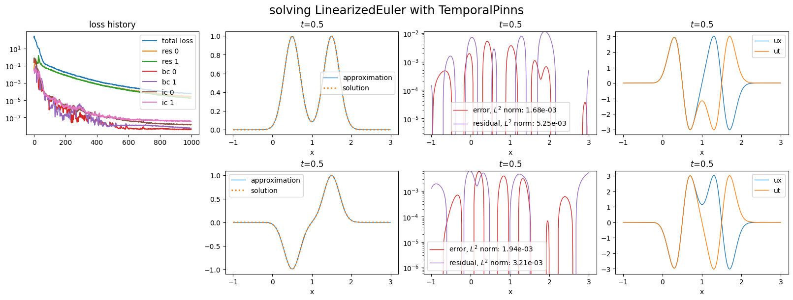
[18]:
plot_abstract_approx_spaces(
    pinn.space,
    domain_x,
    domain_mu,
    domain_t,
    time_values=[
        t_max,
    ],
    loss=pinn.losses,
    residual=pde,
    solution=exact_solution,
    error=exact_solution,
    derivatives=["ux", "ut"],
    title="solving LinearizedEuler with TemporalPinns",
)

plt.show()
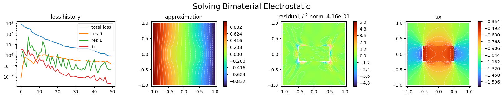
1-dimensional unknown function of space in non-homogeneous medium
We consider in this section a electrostatic problem which consist in solving a lagrangian on a domain composed of two nested rectangles: \(\Omega_{o} := [-1, 1]\times[-1, 1]\) and \(\Omega_{i} := [-1/2, 1/2]\times[-1/4, 1/4]\) representing two different materials.
The problem is:
with boundary conditions on \(\partial \Omega_{o}\):
with a discontinuity of \(\frac{\partial}{\partial x}u\) and \(\frac{\partial}{\partial y}u\) on \(\partial \Omega_{i}\):
We first define the geometric domains \(\Omega_{o}\) and \(\Omega_{i}\) as sub-domains of a Scimba domain representing \(\Omega\):
[19]:
import matplotlib.pyplot as plt
import torch

from scimba_torch.domain.meshless_domain.domain_2d import Square2D
from scimba_torch.integration.monte_carlo import DomainSampler, TensorizedSampler
from scimba_torch.integration.monte_carlo_parameters import UniformParametricSampler

domain_mu = []
domain_x = Square2D([(-1, 1), (-1, 1)], is_main_domain=True)
domain_x_in = Square2D([(-0.5, 0.5), (-0.25, 0.25)], is_main_domain=False)
domain_x.add_subdomain(domain_x_in)

sampler = TensorizedSampler(
    [DomainSampler(domain_x), UniformParametricSampler(domain_mu)]
)
calls to sampler.sample will return LabelTensor of points with labels:
\(0\) for points in \(\Omega_{o}\setminus\Omega_{i}\),
\(1\) for points in \(\Omega_{i}\),
while calls to sampler.sample will return LabelTensor of points with labels:
\(0\) for points in \(\{x,y \in \Omega_{o} | y = -1 \}\),
\(1\) for points in \(\{x,y \in \Omega_{o} | x = 1 \}\),
\(2\) for points in \(\{x,y \in \Omega_{o} | y = 1 \}\),
\(3\) for points in \(\{x,y \in \Omega_{o} | x = -1 \}\),
\(100\) for points in \(\{x,y \in \Omega_{i} | y = -1/4 \}\),
\(101\) for points in \(\{x,y \in \Omega_{i} | x = 1/2 \}\),
\(102\) for points in \(\{x,y \in \Omega_{i} | y = 1/4 \}\),
\(103\) for points in \(\{x,y \in \Omega_{i} | x = -1/2 \}\).
To tackle the problem of the discontinuity of the partial derivatives of the unknown \(u\), we will approximate it with an approximation functions with 2 dimensional output, say
where \(u^o_{\theta}\) approximates \(u\) on \(\Omega_o\) and \(u^i_{\theta}\) approximates \(u\) on \(\Omega_i\).
The residual becomes a system of equations:
and we have the boundary conditions:
Let us define an approximation space to represent this approximating function \({\bf u}_{\theta}\):
[20]:
from scimba_torch.approximation_space.nn_space import NNxSpace
from scimba_torch.neural_nets.coordinates_based_nets.mlp import GenericMLP

space = NNxSpace(
    2,  # number of components
    0,  # number of parameters
    GenericMLP,  # type of nn
    domain_x,  # geometric domain
    sampler,  # associated sampler
    layer_sizes=[40, 40],  # layer sizes
)
We define now a class to model our problem:
[21]:
from scimba_torch.physical_models.elliptic_pde.abstract_elliptic_pde import (
    StrongFormEllipticPDE,
)


class BimaterialElectrostatic(StrongFormEllipticPDE):
    def __init__(self, space, f, g, **kwargs):
        super().__init__(
            space,
            linear=True,  # the operator is linear
            residual_size=2,  # the residual has 2 equations
            bc_residual_size=16,  # the residual for boundary condition has 16 equations
            **kwargs,
        )
        self.f = f
        self.g = g
        self.e_r = 3.3

    def rhs(self, w, x, mu):
        return self.f(x, mu)

    def bc_rhs(self, w, x, n, mu):
        return self.g(x, mu)

    def operator(self, w, x, mu) -> tuple[torch.Tensor, torch.Tensor]:
        u_0, u_1 = w.get_components()  # the 2 components of u
        u_x_0, u_y_0 = self.grad(u_0, x)
        u_xx_0, _ = self.grad(u_x_0, x)
        _, u_yy_0 = self.grad(u_y_0, x)

        u_x_1, u_y_1 = self.grad(u_1, x)
        u_xx_1, _ = self.grad(u_x_1, x)
        _, u_yy_1 = self.grad(u_y_1, x)

        u_xx_0 = w.restrict_to_labels(
            u_xx_0, labels=[0]
        )  # keep the values of u_0 on outter domain
        u_yy_0 = w.restrict_to_labels(u_yy_0, labels=[0])
        u_xx_1 = w.restrict_to_labels(
            u_xx_1, labels=[1]
        )  # keep the values of u_1 on inner domain
        u_yy_1 = w.restrict_to_labels(u_yy_1, labels=[1])

        # return the left hand side of the residuals as 2 elements of a tupple
        return -(u_xx_0 + u_yy_0), -5 * (
            u_xx_1 + u_yy_1
        )  # return the left hand side of the residual

    def bc_operator(
        self, w: MultiLabelTensor, x: LabelTensor, n: LabelTensor, mu: LabelTensor
    ) -> tuple[torch.Tensor, ...]:
        pass  # to be defined later
Here, the operator returns a tuple of 2 torch.Tensor, which are the right hand sides of the 2 equations of the system above.
In order to use natural gradient descent algorithm, one has to define two functional operators, one for each of the labels \(0\) and \(1\), and to store it in an ordered dictionary:
[22]:
from collections import OrderedDict


class BimaterialElectrostatic(BimaterialElectrostatic):
    def restrict_to_component(self, i: int, func):
        return lambda *args: func(*args)[i : i + 1, ...]

    def functional_operator_0(self, func, x, mu, theta):
        grad_u = self.restrict_to_component(0, torch.func.jacrev(func, 0))
        hessian_u = torch.func.jacrev(grad_u, 0)(x, mu, theta)
        return -(hessian_u[..., 0, 0] + hessian_u[..., 1, 1])

    def functional_operator_1(self, func, x, mu, theta):
        grad_u = self.restrict_to_component(1, torch.func.jacrev(func, 0))
        hessian_u = torch.func.jacrev(grad_u, 0)(x, mu, theta)
        return -5.0 * (hessian_u[..., 0, 0] + hessian_u[..., 1, 1])

    def functional_operator(self) -> OrderedDict:
        return OrderedDict(
            [(0, self.functional_operator_0), (1, self.functional_operator_1)]
        )
Let us now see the boundary conditions as a system of 16 equations of which the left hand side is:
[23]:
class BimaterialElectrostatic(BimaterialElectrostatic):
    def bc_operator(
        self, w: MultiLabelTensor, x: LabelTensor, n: LabelTensor, mu: LabelTensor
    ) -> tuple[torch.Tensor, ...]:
        u_o, u_i = w.get_components()
        u_o_x, u_o_y = self.grad(u_o, x)
        u_i_x, u_i_y = self.grad(u_i, x)

        u_o_y_S = w.restrict_to_labels(u_o_y, labels=[0])
        u_o_E = w.restrict_to_labels(u_o, labels=[1])
        u_o_y_N = w.restrict_to_labels(u_o_y, labels=[2])
        u_o_W = w.restrict_to_labels(u_o, labels=[3])

        u_o_i_S = w.restrict_to_labels(u_o, labels=[100])
        u_i_S = w.restrict_to_labels(u_i, labels=[100])
        u_o_i_E = w.restrict_to_labels(u_o, labels=[101])
        u_i_E = w.restrict_to_labels(u_i, labels=[101])
        u_o_i_N = w.restrict_to_labels(u_o, labels=[102])
        u_i_N = w.restrict_to_labels(u_i, labels=[102])
        u_o_i_W = w.restrict_to_labels(u_o, labels=[103])
        u_i_W = w.restrict_to_labels(u_i, labels=[103])

        u_o_i_y_S = w.restrict_to_labels(u_o_y, labels=[100])
        u_i_y_S = w.restrict_to_labels(u_i_y, labels=[100])

        u_o_i_x_E = w.restrict_to_labels(u_o_x, labels=[101])
        u_i_x_E = w.restrict_to_labels(u_i_x, labels=[101])

        u_o_i_y_N = w.restrict_to_labels(u_o_y, labels=[102])
        u_i_y_N = w.restrict_to_labels(u_i_y, labels=[102])

        u_o_i_x_W = w.restrict_to_labels(u_o_x, labels=[103])
        u_i_x_W = w.restrict_to_labels(u_i_x, labels=[103])

        # as we need two equations for each boundary element, we add
        # dummy equations 0 = 0 to boundaries labeled 0, 1, 2, 3.
        return (
            u_o_y_S,
            0 * u_o_y_S,  # the left hand side of an equation 0 = 0
            (u_o_E + 1),  # will give u_o_E = -1
            0 * u_o_E,  # the left hand side of an equation 0 = 0
            u_o_y_N,
            0 * u_o_y_N,  # the left hand side of an equation 0 = 0
            (u_o_W - 1),  # will give u_o_W = 1
            0 * u_o_W,  # the left hand side of an equation 0 = 0
            (u_o_i_S - u_i_S),  # equality of the 2 components on the \partial \Omega_i
            (u_o_i_y_S - self.e_r * u_i_y_S),  # discontinuity of the partial derivative
            (u_o_i_E - u_i_E),  # equality of the 2 components on the \partial \Omega_i
            (u_o_i_x_E - self.e_r * u_i_x_E),  # discontinuity of the partial derivative
            (u_o_i_N - u_i_N),  # equality of the 2 components on the \partial \Omega_i
            (u_o_i_y_N - self.e_r * u_i_y_N),  # discontinuity of the partial derivative
            (u_o_i_W - u_i_W),  # equality of the 2 components on the \partial \Omega_i
            (u_o_i_x_W - self.e_r * u_i_x_W),  # discontinuity of the partial derivative
        )
We now define 8 functional operators for the boundary (1 per label of the boundary), each being the left hand side of a system of 2 equations. The functional operators are stored in a dictionary:
[24]:
class BimaterialElectrostatic(BimaterialElectrostatic):
    def functional_operator_bc_0(self, func, x, n, mu, theta):
        res = 1. * torch.func.jacrev(func, 0)(x, mu, theta)[..., 1]
        res[1, ...] *= 0.0  # the left hand side of an equation 0 = 0
        return res

    def functional_operator_bc_1(self, func, x, n, mu, theta):
        res = func(x, mu, theta) + 1.0
        res[1, ...] *= 0.0  # the left hand side of an equation 0 = 0
        return res

    def functional_operator_bc_2(self, func, x, n, mu, theta):
        return self.functional_operator_bc_0(func, x, n, mu, theta)

    def functional_operator_bc_3(self, func, x, n, mu, theta):
        res = func(x, mu, theta) - 1.0
        res[1, ...] *= 0.0  # the left hand side of an equation 0 = 0
        return res

    def functional_operator_bc_100(self, func, x, n, mu, theta):
        u = func(x, mu, theta)
        u0_m_u1 = u[0:1, ...] - u[1:2, ...]
        grad_u = torch.func.jacrev(func, 0)(x, mu, theta)
        grad_u0_m_grad_u1 = grad_u[0:1, 1] - self.e_r * grad_u[1:2, 1]

        res = torch.cat((5 * u0_m_u1, 1 * grad_u0_m_grad_u1), dim=0)
        return res

    def functional_operator_bc_101(self, func, x, n, mu, theta):
        u = func(x, mu, theta)
        u0_m_u1 = u[0:1, ...] - u[1:2, ...]
        grad_u = torch.func.jacrev(func, 0)(x, mu, theta)
        grad_u0_m_grad_u1 = grad_u[0:1, 0] - self.e_r * grad_u[1:2, 0]

        res = torch.cat((4 * u0_m_u1, 1 * grad_u0_m_grad_u1), dim=0)
        return res

    def functional_operator_bc_102(self, func, x, n, mu, theta):
        return self.functional_operator_bc_100(func, x, n, mu, theta)

    def functional_operator_bc_103(self, func, x, n, mu, theta):
        return self.functional_operator_bc_101(func, x, n, mu, theta)

    def functional_operator_bc(self) -> OrderedDict:
        return OrderedDict(
            [
                (0, self.functional_operator_bc_0),
                (1, self.functional_operator_bc_1),
                (2, self.functional_operator_bc_2),
                (3, self.functional_operator_bc_3),
                (100, self.functional_operator_bc_100),
                (101, self.functional_operator_bc_101),
                (102, self.functional_operator_bc_102),
                (103, self.functional_operator_bc_103),
            ]
        )
One can now define the right hand side functions:
[25]:
from scimba_torch.utils.scimba_tensors import LabelTensor


def f_rhs(x: LabelTensor, mu: LabelTensor) -> tuple[torch.Tensor, torch.Tensor]:
    x_0, _ = x.get_components(label=0)
    x_1, _ = x.get_components(label=1)
    return torch.zeros_like(x_0), torch.zeros_like(x_1)


def f_bc(x: LabelTensor, mu: LabelTensor) -> tuple[torch.Tensor, ...]:
    x_0, _ = x.get_components(label=0)
    x_1, _ = x.get_components(label=1)
    x_2, _ = x.get_components(label=2)
    x_3, _ = x.get_components(label=3)
    x_4, _ = x.get_components(label=100)
    x_5, _ = x.get_components(label=101)
    x_6, _ = x.get_components(label=102)
    x_7, _ = x.get_components(label=103)
    return (
        torch.zeros_like(x_0),
        torch.zeros_like(x_0),
        torch.zeros_like(x_1),
        torch.zeros_like(x_1),
        torch.zeros_like(x_2),
        torch.zeros_like(x_2),
        torch.zeros_like(x_3),
        torch.zeros_like(x_3),
        torch.zeros_like(x_4),
        torch.zeros_like(x_4),
        torch.zeros_like(x_5),
        torch.zeros_like(x_5),
        torch.zeros_like(x_6),
        torch.zeros_like(x_6),
        torch.zeros_like(x_7),
        torch.zeros_like(x_7),
    )
One can now define a PINN and use it to approximate the solution.
Notice the bc_weights argument that allows to balance the respective weights of boundary condition equations, in contrast to bc_weight that balances the weight of all boundary conditions relatively to the residual. It is an OrderedDict which keys are the ones of functional_operator_bc and values are lists of two weights that is one for each equation for a given key.
[26]:
from scimba_torch.numerical_solvers.elliptic_pde.pinns import (
    NaturalGradientPinnsElliptic,
)

pde = BimaterialElectrostatic(space, f=f_rhs, g=f_bc)

bc_weights = OrderedDict(
    [
        (0, [4.0, 0.0]),
        (1, [9.0, 0.0]),
        (2, [4.0, 0.0]),
        (3, [9.0, 0.0]),
        (100, [25.0, 1.0]),
        (101, [16.0, 1.0]),
        (102, [25.0, 1.0]),
        (103, [16.0, 1.0]),
    ]
)

pinns = NaturalGradientPinnsElliptic(
    pde,
    bc_type="weak",
    bc_weight=30.0,
    bc_weights=bc_weights,
    one_loss_by_equation=True,
    matrix_regularization=5e-4,
)
pinns.solve(epochs=50, n_collocation=2000, n_bc_collocation=5000)
Training: 100%|||||||||||||||||||| 50/50[00:29<00:00] , loss: 7.6e+02 -> 8.2e-01
[27]:
from scimba_torch.plots.plots_nd import plot_abstract_approx_spaces

plot_abstract_approx_spaces(
    pinns.space,
    domain_x,
    domain_mu,
    loss=pinns.losses,
    residual=pinns.pde,
    derivatives=["ux"],
    components=[{0: 0, 1: 1}],
    draw_contours=True,
    n_drawn_contours=20,
    # parameters_values="mean",
    title="Solving Bimaterial Electrostatic",
    loss_groups=["bc"],
)
plt.show()