Imposing mixed boundary conditions

In this tutorial, we will solve a 2D Poisson PDE on an annulus with mixed boundary conditions using a Scimba PINNs.

We want to approximate \(u: \Omega \times \mathbb{M} \rightarrow \mathbb{R}\) satisfying

\[\begin{split}\left\{\begin{array}{rl}-\mu \Delta u & = f \text{ in } \Omega \times \mathbb{M} \\ u & = g \text{ on } (\partial \Omega)_0 \times \mathbb{M} \\ \dfrac{\partial u}{\partial {\bf n}} & = h \text{ on } (\partial \Omega)_1 \times \mathbb{M} \\ \end{array}\right.\end{split}\]

where:

• \({\bf x} = (x, y) \in \Omega := \left\{ {\bf x} ~ | ~ r \leq \|{\bf x}\|_2 \leq R \right\}\), \(r=0.2\), \(R=1\),

• \((\partial \Omega)_0 := \left\{ {\bf x} ~ | ~ \|{\bf x}\|_2 = 1 \right\}\),

• \((\partial \Omega)_1 := \left\{ {\bf x} ~ | ~ \|{\bf x}\|_2 = 0.2 \right\}\),

• \(\mu \in \mathbb{M} = [1, 2]\),

• \(f:=1\) and \(g\), \(h\) are identically \(0\).

This problem has the exact solution:

\[u^*({\bf x}, \mu) = \dfrac{r^2}{2\mu} \ln \dfrac{\|{\bf x}\|_2}{R^2} - \dfrac{\left(\|{\bf x}\|_2\right)^2 - R^2}{4\mu}\]

We first define constants.

c = (0.0, 0.0)
r = 0.2
R = 1.0

The parametric domain \(\mathbb{M}\) is defined as a cartesian product of compact intervals of \(\mathbb{R}\):

M = [(1.0, 2.0)]

Geometric domain \(\Omega\)

The difficulties one must face to solve the considered problem are the complex shape of the geometric domain with two boundaries (complex meaning non rectangular), and the boundary conditions that depend on the considered boundary.

Scimba allows the user to implement easily such problems by offering the possibility to construct geometric domains as compositions of simple geometric shapes; subdomains of the geometric domain and of its boundaries are labeled by integers.

Example: creating a 2D disk

from scimba_torch.domain.meshless_domain.domain_2d import Disk2D

# disk centered in c of radius R
Omega = Disk2D(c, R, is_main_domain=True)

The keyword argument is_main_domain indicates whether the created object is a main domain or a subdomain of a main domain.

Here \(\Omega\) is the unit disk - nothing fancy. Its interior is labeled \(0\) and its boundary, the unit circle, is labeled \(0\) (interiors and boundaries are labeled separately).

Creating a 2D annulus

We define \(\Omega\) as \(\mathcal{D}_{out}\setminus \mathcal{D}_{in}\).

We create the disk hole to be attached as a hole to Omega (it is not a main domain):

hole = Disk2D(c, r, is_main_domain=False)

Then

Omega.add_hole(hole)

\(\Omega\) is now the annulus \(\left\{ {\bf x} ~ | ~ r \leq \|{\bf x}\|_2 \leq R \right\}\); the labels are created as subdomains are added to the domain and its boundaries: there is no new label for the interior of Omega, however the boundary of hole has been added to the boundaries of Omega when adding the hole; it is now labeled \(1\).

Sampling the geometric domain \(\Omega\)

Scimba offers ready-to-use uniform samplers for geometric domains and their boundaries:

from scimba_torch.integration.monte_carlo import DomainSampler

sampler_Omega = DomainSampler(Omega)

A domain sampler has two main functionalities: sampling the domain (sample) and sampling the boundaries (bc_sample). The boundary sampler also returns the normals at sampled points:

xy = sampler_Omega.sample(1000)
xy_bc, n_bc = sampler_Omega.bc_sample(2000)

print("xy.shape: ", xy.shape, "xy_bc.shape: ", xy_bc.shape, "n_bc.shape: ", n_bc.shape)

xy.shape:  torch.Size([1000, 2]) xy_bc.shape:  torch.Size([2000, 2]) n_bc.shape:  torch.Size([2000, 2])

The samples returned by samplers are LabelTensors, that are pairs formed of two batched torch.Tensor; one of points and one of associated labels:

print("0-th point: ", xy_bc.x[0], ", label: ", xy_bc.labels[0], " normals: ", n_bc.x[0])
print("\na point with label 1:")
(xy_bc.x[xy_bc.labels == 1])[0]

0-th point:  tensor([-0.9608, -0.2773], grad_fn=<SelectBackward0>) , label:  tensor(0, dtype=torch.int32)  normals:  tensor([-0.9608, -0.2773], grad_fn=<SelectBackward0>)

a point with label 1:

tensor([-0.0336, -0.1972], grad_fn=<SelectBackward0>)

One can retrieve the components for given labels:

x, y = xy.get_components()
x_bc0, y_bc0 = xy_bc.get_components(label=0)
x_bc1, y_bc1 = xy_bc.get_components(label=1)

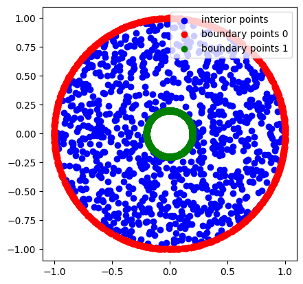
Let us plot the sampled points.

x = x.cpu().detach().numpy()
y = y.cpu().detach().numpy()
x_bc0 = x_bc0.cpu().detach().numpy()
y_bc0 = y_bc0.cpu().detach().numpy()
x_bc1 = x_bc1.cpu().detach().numpy()
y_bc1 = y_bc1.cpu().detach().numpy()

import matplotlib.pyplot as plt

fig = plt.figure()
axe = fig.add_subplot(1, 1, 1)
axe.scatter(x, y, color="b", label="interior points")
axe.scatter(x_bc0, y_bc0, color="r", label="boundary points 0")
axe.scatter(x_bc1, y_bc1, color="g", label="boundary points 1")
axe.set_aspect("equal")
axe.legend()
plt.show()

Sampling \(\Omega\times \mathbb{M}\)

Below we will need a sampler for \(\Omega\times \mathbb{M}\); this is done in Scimba as follows:

from scimba_torch.integration.monte_carlo import TensorizedSampler
from scimba_torch.integration.monte_carlo_parameters import UniformParametricSampler

sampler_M = UniformParametricSampler(M)
sampler = TensorizedSampler([sampler_Omega, sampler_M])

# sample Omega and its boundary
N = 1000
N_bc = 1000
xy, mu = sampler.sample(N)
(xy_bc, n_bc), mu_bc = sampler.bc_sample(N_bc, index_bc=0)

Approximation space

It is time to define the approximation space where we will search for an approximation of the solution as a function \(u_{\theta} : \Omega\times \mathbb{M} \rightarrow \mathbb{R}\).

Neural net based approximation spaces defined on a geometric domain and a parametric domain are implemented in Scimba by the class NNxSpace:

from scimba_torch.approximation_space.nn_space import NNxSpace
from scimba_torch.neural_nets.coordinates_based_nets.mlp import GenericMLP

u_theta = NNxSpace(
    1,  # the output dimension
    1,  # the parameter's space dimension
    GenericMLP,  # the type of neural network, here a MLP
    Omega,  # the geometric domain
    sampler,  # the sampler
    layer_sizes=[64],  # the size of intermediate layers
)

# evaluate NNxSpace on x, mu:
w = u_theta.evaluate(xy, mu)
w.shape

torch.Size([1000, 1])

Evaluation of a NNxSpace returns a MultiLabelTensor which allows, among others, to handle the label information:

w_bc = u_theta.evaluate(xy_bc, mu_bc)

u_bc_ou = w_bc.restrict_to_labels(labels=[0])
u_bc_in = w_bc.restrict_to_labels(labels=[1])

assert u_bc_ou.shape[0] + u_bc_in.shape[0] == w_bc.shape[0]

Get w as a torch.Tensor with:

u = w.get_components()
u.shape

torch.Size([1000, 1])

One compute gradients of u_theta with:

u_x, u_y = u_theta.grad(w, xy)

for boundary data:

u_x_bc, u_y_bc = u_theta.grad(w_bc, xy_bc)

u_x_in = w_bc.restrict_to_labels(u_x_bc, labels=[1])
u_y_in = w_bc.restrict_to_labels(u_y_bc, labels=[1])

Implementation of the model

We will now implement our problem:

\[\begin{split}\left\{\begin{array}{rl}-\mu \Delta u & = f \text{ in } \Omega \times \mathbb{M} \\ u & = g \text{ on } (\partial \Omega)_0 \times \mathbb{M} \\ \dfrac{\partial u}{\partial {\bf n}} & = h \text{ on } (\partial \Omega)_1 \times \mathbb{M} \\ \end{array}\right.\end{split}\]

Interior condition

Below is a function implementing the right-hand side of the first equation:

import torch
from scimba_torch.utils.scimba_tensors import LabelTensor, MultiLabelTensor

def f_rhs(xy: LabelTensor, mu: LabelTensor) -> torch.Tensor:
    x, _ = xy.get_components()
    return torch.ones_like(x)

The following function implements the left-hand side of the first equation:

from scimba_torch.approximation_space.abstract_space import AbstractApproxSpace

def interior_operator(
    space: AbstractApproxSpace, w: MultiLabelTensor, xy: LabelTensor, mu: LabelTensor
) -> torch.Tensor:
    u = w.get_components()
    mu = mu.get_components()
    # compute u_xx and u_yy,
    # the second order derivatives with respect to x and y
    u_x, u_y = space.grad(u, xy)
    u_xx, _ = space.grad(u_x, xy)
    _, u_yy = space.grad(u_y, xy)
    return -mu * (u_xx + u_yy)

Run the code below to check your implementation:

xy, mu = sampler.sample(N)
w = u_theta.evaluate(xy, mu)
L = interior_operator(u_theta, w, xy, mu)
assert L.shape == (N, 1)

def exact_sol(xy: LabelTensor, mu: LabelTensor, r=r, R=R) -> MultiLabelTensor:
    x, y = xy.get_components()
    mu = mu.get_components()
    xynorm = torch.sqrt(x**2 + y**2)
    res = (r**2 / (2 * mu)) * torch.log(xynorm / R)
    res -= (1.0 / (4 * mu)) * (xynorm**2 - R**2)
    return MultiLabelTensor(res, [xy.labels])


class mspace:
    def grad(
        self, u: torch.Tensor | MultiLabelTensor, x: torch.Tensor | LabelTensor
    ) -> torch.Tensor:
        if isinstance(u, MultiLabelTensor):
            u = u.w
        if isinstance(x, LabelTensor):
            x = x.x
        (dudx,) = torch.autograd.grad(u, x, torch.ones_like(u), create_graph=True)
        if x.size(1) > 1:
            return (dudx[:, i, None] for i in range(x.size(1)))
        else:
            return dudx[:, 0, None]


w = exact_sol(xy, mu)
uspace = mspace()

assert torch.allclose(interior_operator(uspace, w, xy, mu), torch.ones_like(w.w))

Boundary conditions

We will now implement the boundary conditions of our model, that is:

\[\begin{split}\left\{\begin{array}{rl} u & = g \text{ on } (\partial \Omega)_0 \times \mathbb{M} \\ \dfrac{\partial u}{\partial {\bf n}} & = h \text{ on } (\partial \Omega)_1 \times \mathbb{M} \\ \end{array}\right.\end{split}\]

For this, we will implement functions computing respectively the left-hand side and the right-hand side of these two equations, and returning tuples (one element by equation).

Below is a function for computing the right-hand side:

def gh_rhs(xy: LabelTensor, mu: LabelTensor) -> tuple[torch.Tensor, torch.Tensor]:
    x_ou, _ = xy.get_components(label=0)
    x_in, _ = xy.get_components(label=1)
    return torch.zeros_like(x_ou), torch.zeros_like(x_in)

The following function implements the left-hand side of the boundary conditions; notice the use of restrict_to_labels to get values of the approximation on appropriated labels:

def boundary_operator(
    space: AbstractApproxSpace,
    w: MultiLabelTensor,
    xy: LabelTensor,
    n: LabelTensor,
    mu: LabelTensor,
) -> tuple[torch.Tensor, torch.Tensor]:
    # Dirichlet condition on outer circle
    u_ou = w.restrict_to_labels(labels=[0])
    # Neumann condition on inner circle
    u = w.get_components()
    u_x, u_y = space.grad(u, xy)
    u_x_in = w.restrict_to_labels(u_x, labels=[1])
    u_y_in = w.restrict_to_labels(u_y, labels=[1])
    nx_in, ny_in = n.get_components(label=1)
    u_in = u_x_in * nx_in + u_y_in * ny_in
    # return a tuple
    return u_ou, u_in

Run the code below to check your implementation:

(xy_bc, n_bc), mu_bc = sampler.bc_sample(N_bc, index_bc=0)
w_bc = u_theta.evaluate(xy_bc, mu_bc)
L0, L1 = boundary_operator(u_theta, w_bc, xy_bc, n_bc, mu_bc)
R0, R1 = gh_rhs(xy_bc, mu_bc)
assert L0.shape == R0.shape
assert L1.shape == R1.shape

w_bc = exact_sol(xy_bc, mu_bc)
L0, L1 = boundary_operator(uspace, w_bc, xy_bc, n_bc, mu_bc)
R0, R1 = gh_rhs(xy_bc, mu_bc)
assert torch.allclose(L0, R0)
assert torch.allclose(L1, R1)

ScimBa model

We now provide the ScimBa implementation for the considered problem, which angular stones are interior and boundary operators.

from scimba_torch.physical_models.elliptic_pde.abstract_elliptic_pde import (
    StrongFormEllipticPDE,
)


class Laplacian2DMixedBCStrongForm(StrongFormEllipticPDE):
    def __init__(self, space: AbstractApproxSpace, **kwargs):
        super().__init__(space, residual_size=1, bc_residual_size=2, **kwargs)

    def rhs(
        self, w: MultiLabelTensor, xy: LabelTensor, mu: LabelTensor
    ) -> torch.Tensor:
        return f_rhs(xy, mu)

    def operator(
        self, w: MultiLabelTensor, xy: LabelTensor, mu: LabelTensor
    ) -> torch.Tensor:
        return interior_operator(self.space, w, xy, mu)

    def bc_rhs(
        self, w: MultiLabelTensor, xy: LabelTensor, n: LabelTensor, mu: LabelTensor
    ) -> tuple[torch.Tensor, torch.Tensor]:
        return gh_rhs(xy, mu)

    def bc_operator(
        self, w: MultiLabelTensor, xy: LabelTensor, n: LabelTensor, mu: LabelTensor
    ) -> tuple[torch.Tensor, torch.Tensor]:
        return boundary_operator(self.space, w, xy, n, mu)

Let us instantiate it:

pde = Laplacian2DMixedBCStrongForm(u_theta)

Approximate the solution with a PINNs

So far, we defined:

M = [(1.0, 2.0)]
Omega = Disk2D((0.0, 0.0), R, is_main_domain=True)
Omega.add_hole(Disk2D((0.0, 0.0), r))

sampler = TensorizedSampler([DomainSampler(Omega), UniformParametricSampler(M)])

u_theta = NNxSpace(1, 1, GenericMLP, Omega, sampler, layer_sizes=[64])

pde = Laplacian2DMixedBCStrongForm(u_theta)

We will now use a Scimba PINNs to approximate the solution of our problem:

from scimba_torch.numerical_solvers.elliptic_pde.pinns import PinnsElliptic

pinn = PinnsElliptic(
    pde,
    bc_type="weak",  # handle weakly the boundary conditions
    bc_weight=10.0,  # balance loss of the boundary conditions / residual
    one_loss_by_equation=True,
)

import timeit

start = timeit.default_timer()
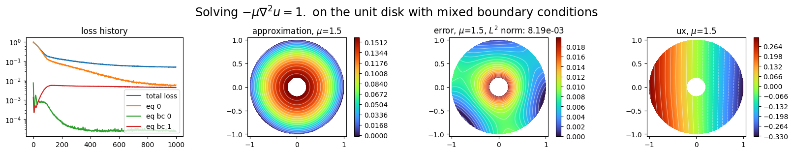
pinn.solve(epochs=1000, n_collocation=2000, n_bc_collocation=4000, verbose=False)
end = timeit.default_timer()

print("loss after optimization: ", pinn.best_loss)
print("approximation time: %f s" % (end - start))

Training: 100%|||||||||||||||| 1000/1000[00:12<00:00] , loss: 9.7e-01 -> 4.8e-02
loss after optimization:  0.04762082480136851
approximation time: 12.476625 s

Plot the approximation:

from scimba_torch.plots.plots_nd import plot_abstract_approx_spaces


def ustar(xy: LabelTensor, mu: LabelTensor, r=r, R=R) -> MultiLabelTensor:
    x, y = xy.get_components()
    mu = mu.get_components()
    xynorm = torch.sqrt(x**2 + y**2)
    res = (r**2 / (2 * mu)) * torch.log(xynorm / R)
    res -= (1.0 / (4 * mu)) * (xynorm**2 - R**2)
    return res


plot_abstract_approx_spaces(
    pinn.space,
    Omega,
    M,
    loss=pinn.losses,
    # residual=pinn.pde,
    draw_contours=True,
    n_drawn_contours=20,
    error=ustar,
    derivatives=["ux"],
    parameters_values="mean",
    title=r"Solving $-\mu\nabla^2 u = 1.$ on the unit disk with mixed boundary conditions",
    n_visu=512,
)
plt.show()

Use Natural Gradient Preconditioning:

In order to use Natural Gradient Preconditioned gradient descent, one need to define additional methods as explained in a previous tutorial.

For the functional form of the boundary condition operator, one needs to define one function per subdomain of boundary and to gather them in a dictionary, as demonstrated below:

from collections import OrderedDict


class Laplacian2DMixedBCStrongForm(Laplacian2DMixedBCStrongForm):

    def functional_operator(self, func, x, mu, theta):
        grad_u = torch.func.jacrev(func, 0)
        hessian_u = torch.func.jacrev(grad_u, 0, chunk_size=None)(x, mu, theta)
        return -mu[0] * (hessian_u[..., 0, 0] + hessian_u[..., 1, 1])

    def functional_operator_bc_0(self, func, x, n, mu, theta):
        return func(x, mu, theta)

    def functional_operator_bc_1(self, func, x, n, mu, theta):
        grad_u = torch.func.jacrev(func, 0)(x, mu, theta)
        grad_u_dot_n = grad_u @ n
        return grad_u_dot_n

    def functional_operator_bc(self) -> OrderedDict:
        return OrderedDict(
            [(0, self.functional_operator_bc_0), (1, self.functional_operator_bc_1)]
        )

Let us try it:

u_theta2 = NNxSpace(1, 1, GenericMLP, Omega, sampler, layer_sizes=[64])

pde2 = Laplacian2DMixedBCStrongForm(u_theta2)

from scimba_torch.numerical_solvers.elliptic_pde.pinns import (
    NaturalGradientPinnsElliptic,
)

pinn2 = NaturalGradientPinnsElliptic(
    pde2,
    bc_type="weak",  # handle weakly the boundary conditions
    bc_weight=30.0,  # balance loss of the boundary conditions / residual
    bc_weights=OrderedDict(
        [(0, 1.0), (1, 1.0)]
    ),  # balance losses of the boundary conditions
    one_loss_by_equation=True,
)

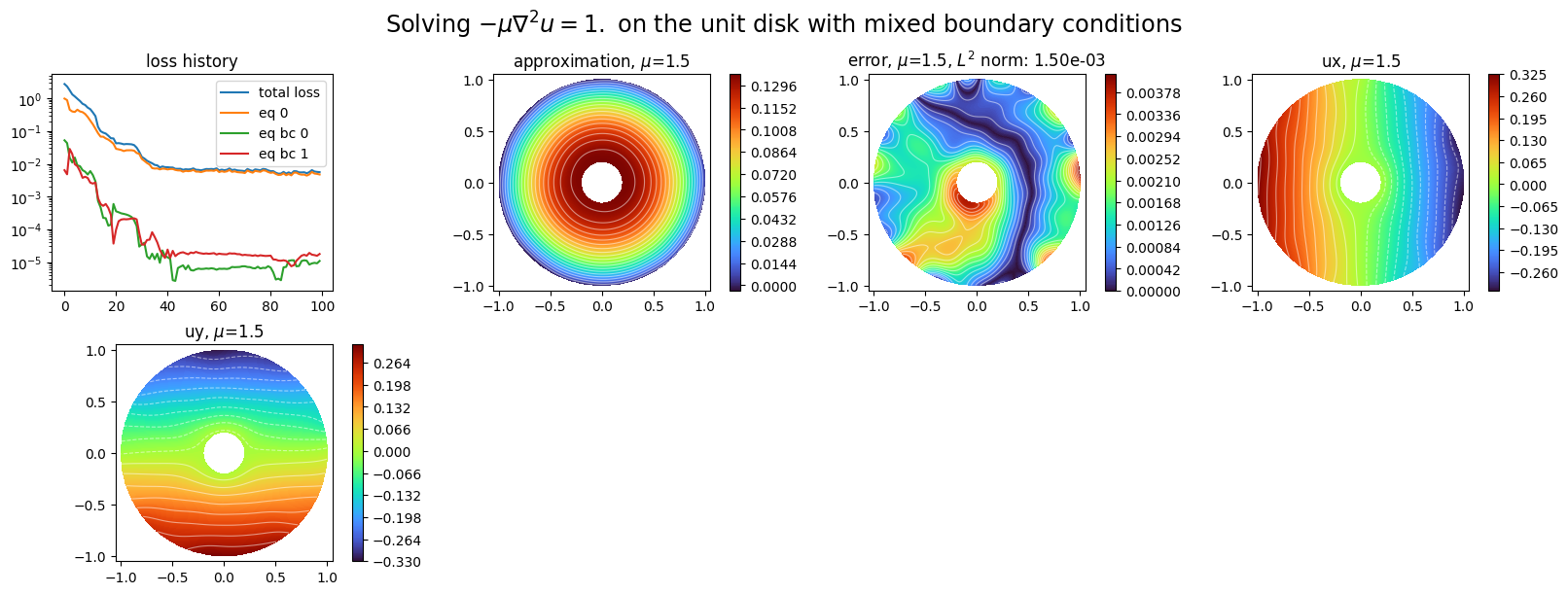
start = timeit.default_timer()
pinn2.solve(epochs=100, n_collocation=2000, n_bc_collocation=4000, verbose=False)
end = timeit.default_timer()

print("loss after optimization: ", pinn2.best_loss)
print("approximation time: %f s" % (end - start))

Training: 100%|||||||||||||||||| 100/100[00:04<00:00] , loss: 2.8e+00 -> 5.0e-03
loss after optimization:  0.004997275952951608
approximation time: 4.824741 s

plot_abstract_approx_spaces(
    pinn2.space,
    Omega,
    M,
    loss=pinn2.losses,
    draw_contours=True,
    n_drawn_contours=20,
    error=ustar,
    derivatives=["ux", "uy"],
    parameters_values="mean",
    title=r"Solving $-\mu\nabla^2 u = 1.$ on the unit disk with mixed boundary conditions",
    n_visu=512,
)
plt.show()