Projection of a function on an approximation space.

We demonstrate here how to approximate a known function with a neural network in Scimba on 2 examples. The function to be approximated has to be known as a procedure for its evaluation.

First example: highly curved function

Let

\[f({\bf x}, \mu) = \sin(\theta) \cos(\theta) \exp\left(-\frac{(\theta - \frac{\pi}{4})^2}{2 \sigma_\theta^2}\right) \exp\left(-\frac{(r - 0.5)^2}{2 \sigma_r^2}\right) + 1.1 \cdot \sin(1.5\theta) \cos(0.5\theta) \exp\left(-\frac{0.5 (\theta - \frac{\pi}{4})^2}{2 \sigma_\theta^2}\right) \exp\left(-\frac{1.25 (r - 0.5)^2}{2 \sigma_r^2}\right)\]

where:

\[{\bf x} = (x, y), \quad r' = \sqrt{x^2 + y^2}, \quad \theta = \arctan\left(\frac{y}{x}\right), \quad r = r' + 0.05 \cos(4\pi \theta),\]

\[\sigma_\theta = 0.53, \quad \sigma_r = 0.008.\]

Let us import the required libraries and modules then implement the function to approximate:

import matplotlib.pyplot as plt
import torch

from scimba_torch.utils.scimba_tensors import LabelTensor

def func(x: LabelTensor, mu: LabelTensor):
    x1, x2 = x.get_components()
    r = torch.sqrt(x1**2 + x2**2)
    theta = torch.atan(x2 / x1)
    r = r + 0.05 * torch.cos(4 * torch.pi * theta)
    sigma_theta = 0.53
    sigma_r = 0.008
    return (
        torch.sin(theta)
        * torch.cos(theta)
        * torch.exp(-((theta - torch.pi / 4) ** 2) / (2 * sigma_theta**2.0))
        * torch.exp(-((r - 0.5) ** 2) / (2 * sigma_r**2.0))
    ) + 1.1 * (
        torch.sin(1.5 * theta)
        * torch.cos(0.5 * theta)
        * torch.exp(-0.5 * ((theta - torch.pi / 4) ** 2) / (2 * sigma_theta**2.0))
        * torch.exp(-1.25 * ((r - 0.5) ** 2) / (2 * sigma_r**2.0))
    )

We will approximate this function on the domain \(\Omega = [0, 1] \times [0,1]\):

from scimba_torch.domain.meshless_domain.domain_2d import Square2D
from scimba_torch.integration.monte_carlo import DomainSampler, TensorizedSampler
from scimba_torch.integration.monte_carlo_parameters import UniformParametricSampler

omega = Square2D([(0, 1), (0, 1)], is_main_domain=True)
sampler = TensorizedSampler([DomainSampler(omega), UniformParametricSampler([])])

The base method: projection on a generic MLP based approximation space

We first do as if we had no knowledge of the function to approximate and search an approximation on a NN with a generic MLP architecture:

from scimba_torch.approximation_space.nn_space import NNxSpace
from scimba_torch.neural_nets.coordinates_based_nets.mlp import GenericMLP

space1 = NNxSpace(1, 0, GenericMLP, omega, sampler, layer_sizes=[18, 18])

The parameters of the NN have to be tuned to get an approximation of the desired function; this is what we call projection on the approximation space. To this end, we define a so-called projector:

from scimba_torch.numerical_solvers.collocation_projector import NaturalGradientProjector

p1 = NaturalGradientProjector(space1, func)

Here we use a projector with natural gradient preconditioning, i.e. with natural gradient preconditioned gradient descent. The projection is computed by calling the solve method of the projector:

p1.solve(epochs=400, n_collocation=10000)

Training: 100%|||||||||||||||||| 400/400[00:12<00:00] , loss: 1.1e-02 -> 2.5e-06

Plot the approximation with:

import matplotlib.pyplot as plt
from scimba_torch.plots.plots_nd import plot_abstract_approx_spaces

plot_abstract_approx_spaces(
    p1.space,
    omega,
    loss=p1.losses,
    solution=func,
    error=func,
    draw_contours=True,
    n_drawn_contours=20,
    title="Projection with Energy Natural Gradient",
)

plt.show()

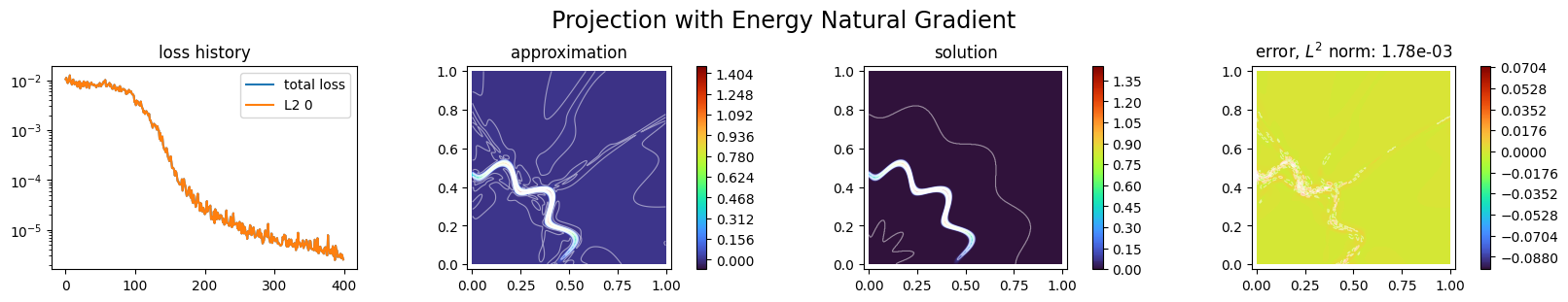
This approach suits well to the case where the function to be approximated is given as a black-box function.

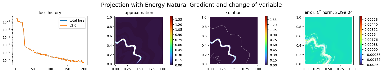
Adapt the network architecture to the function to approximate

In the present case where we know a formula for the function to be approximated, we can take advantage of it.

Remarking that the function we want to approximate is essentially a function of \(\theta\) and \(r\) where:

\[r' = \sqrt{x^2 + y^2}, \quad \theta = \arctan\left(\frac{y}{x}\right), \quad r = r' + 0.05 \cos(4\pi \theta),\]

we propose to apply a change of variable to feed the network with \(\theta\) and \(r\). To this end, we apply a pre-processing to the input of the approximation space:

def variable_change(x, mu):
    x1, x2 = x.get_components()
    r = torch.sqrt(x1**2 + x2**2)
    theta = torch.atan2(x2, x1)
    r = r + 0.05 * torch.cos(4 * torch.pi * theta)
    return torch.cat([r, theta], dim=1)

space2 = NNxSpace(1, 0, GenericMLP, omega, sampler, layer_sizes=[18, 18], pre_processing=variable_change)

p2 = NaturalGradientProjector(space2, func)
p2.solve(epochs=200, n_collocation=10000)

Training: 100%|||||||||||||||||| 200/200[00:06<00:00] , loss: 2.8e-02 -> 4.1e-08

plot_abstract_approx_spaces(
    p2.space,
    omega,
    loss=p2.losses,
    solution=func,
    error=func,
    draw_contours=True,
    n_drawn_contours=20,
    title="Projection with Energy Natural Gradient and change of variable",
)

plt.show()

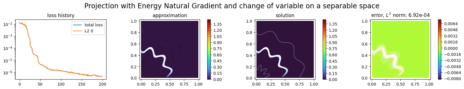
Finally, since the function to approximate is the sum of two quantities, we try to compute its approximation with to MLP-like NNs which outputs are gathered; this can be done with a SeparatedNNxSpace approximation space:

from scimba_torch.approximation_space.nn_space import SeparatedNNxSpace

space3 = SeparatedNNxSpace(
    1,
    0,
    2, # the number of NNs
    GenericMLP,
    omega,
    sampler,
    layer_sizes=[12, 12],
    pre_processing=variable_change,
)

p3 = NaturalGradientProjector(space3, func)
p3.solve(epochs=200, n_collocation=10000)

Training: 100%|||||||||||||||||| 200/200[00:16<00:00] , loss: 1.4e-02 -> 4.3e-07

plot_abstract_approx_spaces(
    p3.space,
    omega,
    loss=p3.losses,
    solution=func,
    error=func,
    draw_contours=True,
    n_drawn_contours=20,
    title="Projection with Energy Natural Gradient and change of variable on a separable space",
)

plt.show()

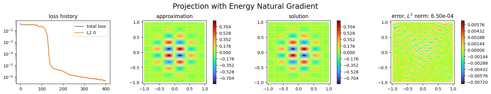
Second example: learning an oscillatory function

We now consider the function:

\[f({\bf x}) = \sin(2.5\pi x) \cdot \sin(4.5\pi y) \cdot \exp\left(-\frac{x^2 + y^2}{2 \sigma^2}\right),\]

where \({\bf x}=(x, y)\) and \(\sigma = 0.4\).

We want to learn \(f\) on \(\Omega = [-1, 1]\times [-1, 1]\).

def func(xy: LabelTensor, mu: LabelTensor):
    x, y = xy.get_components()
    sigma = 0.4
    return (
        torch.sin(2.5 * torch.pi * x)
        * torch.sin(4.5 * torch.pi * y)
        * torch.exp(-((x) ** 2 + (y) ** 2) / (2 * sigma**2))
    )

omega = Square2D([(-1.0, 1.0), (-1.0, 1.0)], is_main_domain=True)
sampler = TensorizedSampler([DomainSampler(omega), UniformParametricSampler([])])

The base method: projection on a generic MLP based approximation space

As previously, we first do as if we had no knowledge on the function to approximate, and project it on a MLP like network:

torch.manual_seed(0)

space1 = NNxSpace(1, 0, GenericMLP, omega, sampler, layer_sizes=[18, 18])
p1 = NaturalGradientProjector(space1, func)
p1.solve(epochs=400, n_collocation=10000)

Training: 100%|||||||||||||||||| 400/400[00:11<00:00] , loss: 4.0e-02 -> 4.2e-07

Remark: the training is a stochastic process; try to change the seed if it does not improve the loss.

plot_abstract_approx_spaces(
    p1.space,
    omega,
    loss=p1.losses,
    solution=func,
    error=func,
    draw_contours=True,
    n_drawn_contours=20,
    title="Projection with Energy Natural Gradient",
)

plt.show()

Adapt the network architecture to the function to approximate

Let us now project the function on a space with Fourier modes. Such an approximation space can be instantiated with:

from scimba_torch.approximation_space.spectral_space import SpectralxSpace

space2 = SpectralxSpace(
    1, # nb of unknowns
    "sine", # basis functions
    6, # nb of modes per direction
    omega.bounds, # domain bounds
    sampler # sampler
)

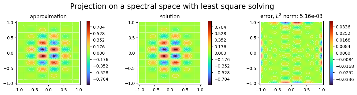
We first propose to adjust the parameters with a least squares solver:

from scimba_torch.numerical_solvers.collocation_projector import LinearProjector

p2 = LinearProjector(space2, func)
p2.solve(n_collocation=10000, verbose=True)

Training done!
    Final loss value: 2.608e-05
     Best loss value: 2.850e-05

plot_abstract_approx_spaces(
    p2.space,
    omega,
    solution=func,
    error=func,
    draw_contours=True,
    n_drawn_contours=20,
    title="Projection on a spectral space with least square solving",
)

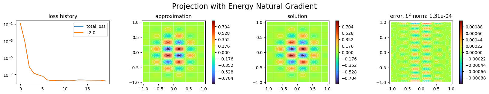
We finally project the function with Natural Gradient preconditioning:

space3 = SpectralxSpace(
    1, # nb of unknowns
    "sine", # basis functions
    6, # nb of modes per direction
    omega.bounds, # domain bounds
    sampler # sampler
)

p3 = NaturalGradientProjector(space3, func)
p3.solve(epochs=20, n_collocation=10000)

Training: 100%|||||||||||||||||||| 20/20[00:00<00:00] , loss: 1.2e-01 -> 1.7e-08

plot_abstract_approx_spaces(
    p3.space,
    omega,
    loss=p3.losses,
    solution=func,
    error=func,
    draw_contours=True,
    n_drawn_contours=20,
    title="Projection with Energy Natural Gradient",
)

plt.show()