Scimba Optimizers
This tutorial presents the optimizers available in Scimba and their use on a simple example.
Scimba proposes:
state-of-the-art generic optimizers:
Adam,SGD, andL-BFGSthat are directly taken frompytorch;two Quasi-Newton methods:
SSBFGSandSSBroydenadapted to PINNs taken from [USP2025]four natural gradient preconditioning methods: Energy Natural Gradient (ENG) [MZ2023], ANaGram [SF2024], Sketchy Natural Gradient (SNG) [MKGVW2025] and Nyström Natural Gradient (NNG) [BMS2025].
SSBFGS and SSBroyden need to update at each step a \(p\times p\) matrix \(H\) (\(p\) being the number of degrees of freedom of the NN).
Natural Gradient based preconditioning require an approximate solution of \(Gx=y\) where \(G\) is of size called energy Gram matrix. Approaches differ in how the approximate solution is computed.
Example
We will illustrate the use of Scimba optimizers on the simple 2D laplacian problem of the first tutorial.
[1]:
import scimba_torch
import torch

from scimba_torch.utils.scimba_tensors import LabelTensor
from scimba_torch.domain.meshless_domain.domain_2d import Square2D
from scimba_torch.integration.monte_carlo import DomainSampler, TensorizedSampler
from scimba_torch.integration.monte_carlo_parameters import UniformParametricSampler
from scimba_torch.approximation_space.nn_space import NNxSpace
from scimba_torch.neural_nets.coordinates_based_nets.mlp import GenericMLP
from scimba_torch.physical_models.elliptic_pde.laplacians import (
    Laplacian2DDirichletStrongForm,
)
from scimba_torch.numerical_solvers.elliptic_pde.pinns import (
    NaturalGradientPinnsElliptic,
)

def f_rhs(xs: LabelTensor, ms: LabelTensor) -> torch.Tensor:
    x, y = xs.get_components()
    mu = ms.get_components()
    pi = torch.pi
    return 2 * (2.0 * mu * pi) ** 2 * torch.sin(2.0 * pi * x) * torch.sin(2.0 * pi * y)


def f_bc(xs: LabelTensor, ms: LabelTensor) -> torch.Tensor:
    x, _ = xs.get_components()
    return x * 0.0

domain_x = Square2D([(0.0, 1), (0.0, 1)], is_main_domain=True)

domain_mu = [(1.0, 2.0)]

sampler = TensorizedSampler(
    [DomainSampler(domain_x), UniformParametricSampler(domain_mu)]
)

torch.manual_seed(0)

space = NNxSpace(
    1,  # the output dimension
    1,  # the parameter's space dimension
    GenericMLP,  # the type of neural network
    domain_x,  # the geometric domain
    sampler,  # the sampler
    layer_sizes=[64],  # the size of intermediate layers
)

pde = Laplacian2DDirichletStrongForm(space, f=f_rhs, g=f_bc)
Classical PINNs
Let us define PINNs with classical optimizers.
Default setting
PinnsElliptic (and TemporalPinns) use by default Adam optimizer with parameters:
lr= 1e-3 (learning rate)betas= (0.9, 0.999)scheduler
lr_scheduler.StepLRwithgamma= 0.99 andstep_size=20
[2]:
from scimba_torch.numerical_solvers.elliptic_pde.pinns import PinnsElliptic

bc_weight = 40.

pinns = PinnsElliptic(
    pde, bc_type="weak", bc_weight=bc_weight
)

pinns.solve(epochs=1000)
Training: 100%|||||||||||||||| 1000/1000[00:05<00:00] , loss: 9.3e+03 -> 3.2e+03
The low value of \(0.001\) for the learning rate is a safe choice. In some cases it can be increased as it is shown below.
Change optimizer:
User can specify the optimizer to be used in PinnsElliptic and TemporalPinns through the optional argument keyword optimizers which value must be in ["adam", "sgd", "lbfgs", "ssbfgs", "ssbroyden"].
Say you want to use L-BFGS:
[3]:
torch.manual_seed(0)

space1 = NNxSpace(1, 1, GenericMLP, domain_x, sampler, layer_sizes=[64])
pde1 = Laplacian2DDirichletStrongForm(space1, f=f_rhs, g=f_bc)

pinns1 = PinnsElliptic(
    pde1, bc_type="weak", optimizers="lbfgs", bc_weight=bc_weight
)

pinns1.solve(epochs=1000)
Training: 100%|||||||||||||||| 1000/1000[00:16<00:00] , loss: 9.3e+03 -> 2.0e+01
or SSBroyden:
[4]:
torch.manual_seed(0)

space2 = NNxSpace(1, 1, GenericMLP, domain_x, sampler, layer_sizes=[64])
pde2 = Laplacian2DDirichletStrongForm(space2, f=f_rhs, g=f_bc)

pinns2 = PinnsElliptic(
    pde2, bc_type="weak", optimizers="ssbroyden", bc_weight=bc_weight
)

pinns2.solve(epochs=1000)
Training: 100%|||||||||||||||| 1000/1000[00:09<00:00] , loss: 9.3e+03 -> 4.5e-01
or SSBFGS:
[5]:
torch.manual_seed(0)

space3 = NNxSpace(1, 1, GenericMLP, domain_x, sampler, layer_sizes=[64])
pde3 = Laplacian2DDirichletStrongForm(space3, f=f_rhs, g=f_bc)

pinns3 = PinnsElliptic(
    pde3, bc_type="weak", optimizers="ssbfgs", bc_weight=bc_weight
)

pinns3.solve(epochs=1000)
Training: 100%|||||||||||||||| 1000/1000[00:09<00:00] , loss: 9.3e+03 -> 1.8e-01
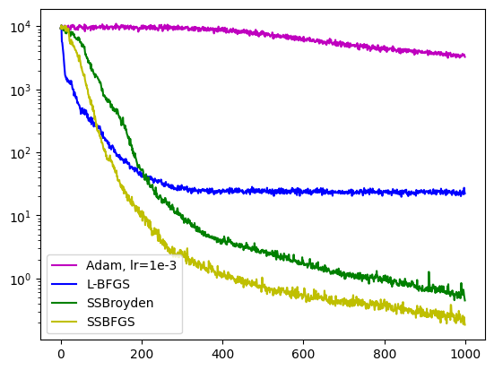
[6]:
import matplotlib.pyplot as plt

fig = plt.figure()
axe = fig.add_subplot(1, 1, 1)

axe.semilogy(pinns.losses.loss_history, label="Adam, lr=1e-3", color='m')
axe.semilogy(pinns1.losses.loss_history, label="L-BFGS", color='b')
axe.semilogy(pinns2.losses.loss_history, label="SSBroyden", color='g')
axe.semilogy(pinns3.losses.loss_history, label="SSBFGS", color='y')
axe.legend()

plt.show()
Optional arguments for optimizers and schedulers
For a more precise control on optimizers arguments, user can give a dict as value to optimizers optional argument. The keys of this dict can be:
"name": mandatory, the name of the optimizer"optimizer_args": optional, arguments for the optimizer"scheduler_args": optional, arguments for the schedulerlr_scheduler.StepLRwhen"name"is"adam"or"sgd"
Let us increase drastically the learning rate for Adam (\(0.018\) instead of \(0.001\)):
[7]:
torch.manual_seed(0)

space4 = NNxSpace(1, 1, GenericMLP, domain_x, sampler, layer_sizes=[64])
pde4 = Laplacian2DDirichletStrongForm(space4, f=f_rhs, g=f_bc)

opt_4 = {
    "name": "adam",
    "optimizer_args": {"lr": 1.8e-2, "betas": (0.9, 0.999)},
}
pinns4 = PinnsElliptic(
    pde4, bc_type="weak", optimizers=opt_4, bc_weight=bc_weight
)

pinns4.solve(epochs=1000)
Training: 100%|||||||||||||||| 1000/1000[00:05<00:00] , loss: 9.3e+03 -> 1.2e+01
Options for Adam, L-BFGS and SGD can be any options accepted by torch their implementation.
SSBFGS and SSBroyden accept options lr (a maximum step size) and tolerance_grad (a stopping criterion on the \(L_\infty\) norm of the gradient).
Combining optimizers
In Scimba, optimizers can be combined to be applied at certain epochs of the optimization process.
Say you want to apply Adam for the first half epochs, then switch to SSBroyden:
[8]:
opt_5 = {
    "name": "ssbroyden",
    "switch_at_epoch_ratio": 0.5
}

space5 = NNxSpace(1, 1, GenericMLP, domain_x, sampler, layer_sizes=[64])
pde5 = Laplacian2DDirichletStrongForm(space5, f=f_rhs, g=f_bc)
pinns5 = PinnsElliptic(
    pde5, bc_type="weak", optimizers=[opt_4, opt_5], bc_weight=bc_weight
)

pinns5.solve(epochs=1000)
Training: 100%|||||||||||||||| 1000/1000[00:07<00:00] , loss: 9.9e+03 -> 2.2e-01
[9]:
fig = plt.figure()
axe = fig.add_subplot(1, 1, 1)
axe.semilogy(pinns5.losses.loss_history, label="Adam + SSBroyden", color='m')
axe.legend()

plt.show()
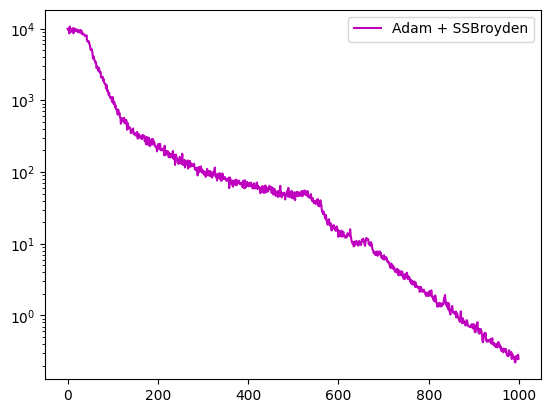
With option switch_at_epoch, one can pass an epoch number rather than a ratio.
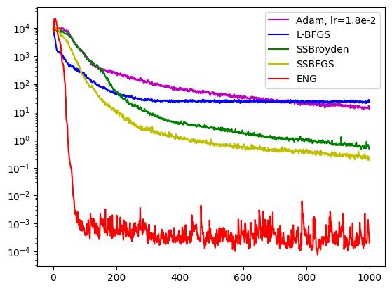
Natural Gradient Preconditioned Gradient Descent
Four Natural Gradient Preconditioned Gradient Descent algorithms are implemented in Scimba and are available through classes
NaturalGradientPinnsEllipticfor stationary problems,NaturalGradientTemporalPinnsfor time dependent problems; the choice of the method in use is done through theng_algokeyword argument; see here and here.
[10]:
from scimba_torch.numerical_solvers.elliptic_pde.pinns import NaturalGradientPinnsElliptic

space6 = NNxSpace(1, 1, GenericMLP, domain_x, sampler, layer_sizes=[64])
pde6 = Laplacian2DDirichletStrongForm(space6, f=f_rhs, g=f_bc)
pinns6 = NaturalGradientPinnsElliptic(
    pde6, bc_type="weak", bc_weight=bc_weight
)

pinns6.solve(epochs=1000)
Training: 100%|||||||||||||||| 1000/1000[00:21<00:00] , loss: 9.3e+03 -> 7.6e-05
[11]:
import matplotlib.pyplot as plt

fig = plt.figure()
axe = fig.add_subplot(1, 1, 1)

axe.semilogy(pinns4.losses.loss_history, label="Adam, lr=1.8e-2", color='m')
axe.semilogy(pinns1.losses.loss_history, label="L-BFGS", color='b')
axe.semilogy(pinns2.losses.loss_history, label="SSBroyden", color='g')
axe.semilogy(pinns3.losses.loss_history, label="SSBFGS", color='y')
axe.semilogy(pinns6.losses.loss_history, label="ENG", color='r')
axe.legend()

plt.show()
References
[USP2025] Urbán, J. F., Stefanou, P., & Pons, J. A. (2025). Unveiling the optimization process of physics informed neural networks: How accurate and competitive can PINNs be?. Journal of Computational Physics, 523, 113656.
[MZ2023] Müller, J., & Zeinhofer, M. (2023, July). Achieving high accuracy with PINNs via energy natural gradient descent. In International Conference on Machine Learning (pp. 25471-25485). PMLR.
[SF2024] Schwencke, N., & Furtlehner, C. (2024). ANAGRAM: a natural gradient relative to adapted model for efficient PINNS learning. arXiv preprint arXiv:2412.10782.
[MKGVW2025] M. Best Mckay, A. Kaur, C. Greif, B. Wetton. Near-optimal Sketchy Natural Gradients for Physics-Informed Neural Networks. Proceedings of the 42nd International Conference on Machine Learning, PMLR 267:4005-4019, 2025.
[BMS2025] I. Bioli, C. Marcati, G. Sangalli. Accelerating Natural Gradient Descent for PINNs with Randomized Nyström Preconditioning. arXiv preprint https://arxiv.org/abs/2505.11638v3