Losses in Scimba PINNs

This tutorial illustrates how the loss is defined in Scimba PINNs (time-dependent or not) and how it can be tuned to improve approximation.

The considered example

The functionalities are illustrated on the linearized euler problem already introduced in this tutorial.

Let us define the model:

from typing import Callable, Tuple

import torch

from scimba_torch.approximation_space.abstract_space import AbstractApproxSpace
from scimba_torch.utils.scimba_tensors import LabelTensor


class LinearizedEuler:
    def __init__(self, space, init, **kwargs):
        self.space = space
        self.init = init

        self.linear = True
        self.residual_size = 2  # the number of equations of the residual
        self.bc_residual_size = 2  # the number of equations of the boundary condition
        self.ic_residual_size = 2  # the number of equations of the initial condition

    def grad(self, w, y):
        return self.space.grad(w, y)

    def rhs(self, w, t, x, mu):
        x_ = x.get_components()
        return torch.zeros_like(x_), torch.zeros_like(x_)

    def bc_rhs(self, w, t, x, n, mu):
        x_ = x.get_components()
        return torch.zeros_like(x_), torch.zeros_like(x_)

    def initial_condition(self, x, mu):
        return self.init(x, mu)  # assume init returns a tuple of 2 tensors

    def time_operator(self, w, t, x, mu):
        u, v = w.get_components()
        u_t = self.grad(u, t)
        v_t = self.grad(v, t)
        return u_t, v_t  # returns a tuple of 2 tensors

    def space_operator(self, w, t, x, mu):
        u, v = w.get_components()
        u_x = self.grad(u, x)
        v_x = self.grad(v, x)
        return v_x, u_x  # returns a tuple of 2 tensors

    def operator(self, w, t, x, mu):
        time_0, time_1 = self.time_operator(w, t, x, mu)
        space_0, space_1 = self.space_operator(w, t, x, mu)
        return time_0 + space_0, time_1 + space_1  # returns a tuple of 2 tensors

    # Dirichlet conditions
    def bc_operator(self, w, t, x, n, mu: LabelTensor):
        u, v = w.get_components()
        return u, v

    def functional_operator(self, u, t, x, mu, theta) -> torch.Tensor:
        # space operator
        u_space = torch.func.jacrev(u, 1)(t, x, mu, theta)
        u_space = torch.flip(u_space, (-1,))
        # time operator
        u_time = torch.func.jacrev(u, 0)(t, x, mu, theta)
        # operator
        res = (u_space + u_time).squeeze()
        return res  # returns a tensor of shape (2,)

    def functional_operator_bc(self, u, t, x, n, mu, theta) -> torch.Tensor:
        return u(t, x, mu, theta)  # returns a tensor of shape (2,)

    def functional_operator_ic(self, u, x, mu, theta) -> torch.Tensor:
        t = torch.zeros_like(x)
        return u(t, x, mu, theta)  # returns a tensor of shape (2,)

def exact_solution(t, x, mu):
    x = x.get_components()
    D = 0.02
    coeff = 1 / (4 * torch.pi * D) ** 0.5
    p_plus_u = coeff * torch.exp(-((x - t.x - 1) ** 2) / (4 * D))
    p_minus_u = coeff * torch.exp(-((x + t.x - 1) ** 2) / (4 * D))
    p = (p_plus_u + p_minus_u) / 2
    u = (p_plus_u - p_minus_u) / 2
    return torch.cat((p, u), dim=-1)

def initial_solution(x, mu):
    sol = exact_solution(LabelTensor(torch.zeros_like(x.x)), x, mu)
    return sol[..., 0:1], sol[..., 1:2]

from scimba_torch.domain.meshless_domain.domain_1d import Segment1D
from scimba_torch.integration.monte_carlo import DomainSampler, TensorizedSampler
from scimba_torch.integration.monte_carlo_parameters import UniformParametricSampler
from scimba_torch.integration.monte_carlo_time import UniformTimeSampler

domain_mu = []
domain_x = Segment1D((-1.0, 3.0), is_main_domain=True)

t_min, t_max = 0.0, 0.5
domain_t = (t_min, t_max)

sampler = TensorizedSampler(
    [
        UniformTimeSampler(domain_t),
        DomainSampler(domain_x),
        UniformParametricSampler(domain_mu),
    ]
)

Define an approximation space (based on a MLP) and instantiate the problem:

from scimba_torch.approximation_space.nn_space import NNxtSpace
from scimba_torch.neural_nets.coordinates_based_nets.mlp import GenericMLP

space = NNxtSpace(2, 0, GenericMLP, domain_x, sampler, layer_sizes=[64])
pde = LinearizedEuler(space, initial_solution)

Default loss used in PINNs

First define a TemporalPinns with SS-BFGS optimizer and weak handling of boundary and initial conditions.

from scimba_torch.numerical_solvers.temporal_pde.pinns import TemporalPinns

pinn = TemporalPinns(
    pde,
    bc_type="weak",
    ic_type="weak",
    one_loss_by_equation=True,
    optimizers="ssbfgs"
)

Notice the one_loss_by_equation optional argument that must be used for approximating solutions of systems of equations.

By default, the loss function \(L\) is defined as:

\[L(\theta) := w_{\text{in}} \sum_i w_{\text{in},i} L_{\text{in},i}(\theta) + w_{\text{bc}} \sum_j w_{\text{bc},j} L_{\text{bc},j}(\theta) + w_{\text{ic}} \sum_k w_{\text{ic},k} L_{\text{ic},k}(\theta) \tag{1}\]

where the default values of the weights are:

\[w_{\text{in}} = 1, w_{\text{bc}}=10, w_{\text{ic}}=10 \text{ and } w_{\text{in},i}, w_{\text{bc},j}, w_{\text{ic},k} = 1 \forall i,j,k\]

and the default loss functions are Mean Squared Errors (MSE): if equation \(i\) of the residual (respectively boundary conditions, initial conditions) is:

\[\mathcal{L}({\bf x}, \theta) = \mathcal{R}({\bf x})\]

then \(L_{\text{in},i}\) (resp. \(L_{\text{bc},j}, L_{\text{ic},k}\)) is defined as

\[L_{\text{in},i}(\theta) = \frac{1}{N}\sum_\ell^N (\mathcal{L}({\bf x}_\ell, \theta) - \mathcal{R}({\bf x}_\ell))^2\]

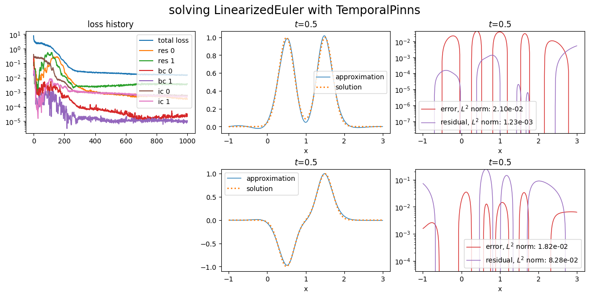
pinn.solve(epochs=1000, n_collocation=3000)

Training: 100%|||||||||||||||| 1000/1000[00:17<00:00] , loss: 3.7e+00 -> 5.0e-05

Plot it; the loss history in the plot gives the values of \(L\), \(L_{\text{in},i}\), \(L_{\text{bc},j}\) and \(L_{\text{ic},k}\) along optimization process:

import matplotlib.pyplot as plt
from scimba_torch.plots.plots_nd import plot_abstract_approx_spaces

plot_abstract_approx_spaces(
    pinn.space,
    domain_x,
    domain_mu,
    domain_t,
    loss=pinn.losses,
    residual=pde,
    solution=exact_solution,
    error=exact_solution,
    title="solving LinearizedEuler with TemporalPinns",
)

plt.show()

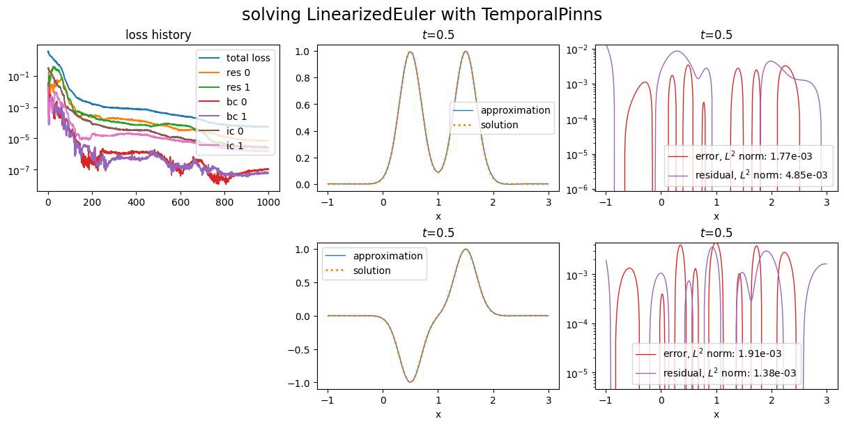
Weights tuning

We first show how to modify the weights used in the computation of the loss (1).

When looking at the values of the losses in the loss history above, one can notice that the losses for the initial conditions are not as well minimized as for the boundary conditions.

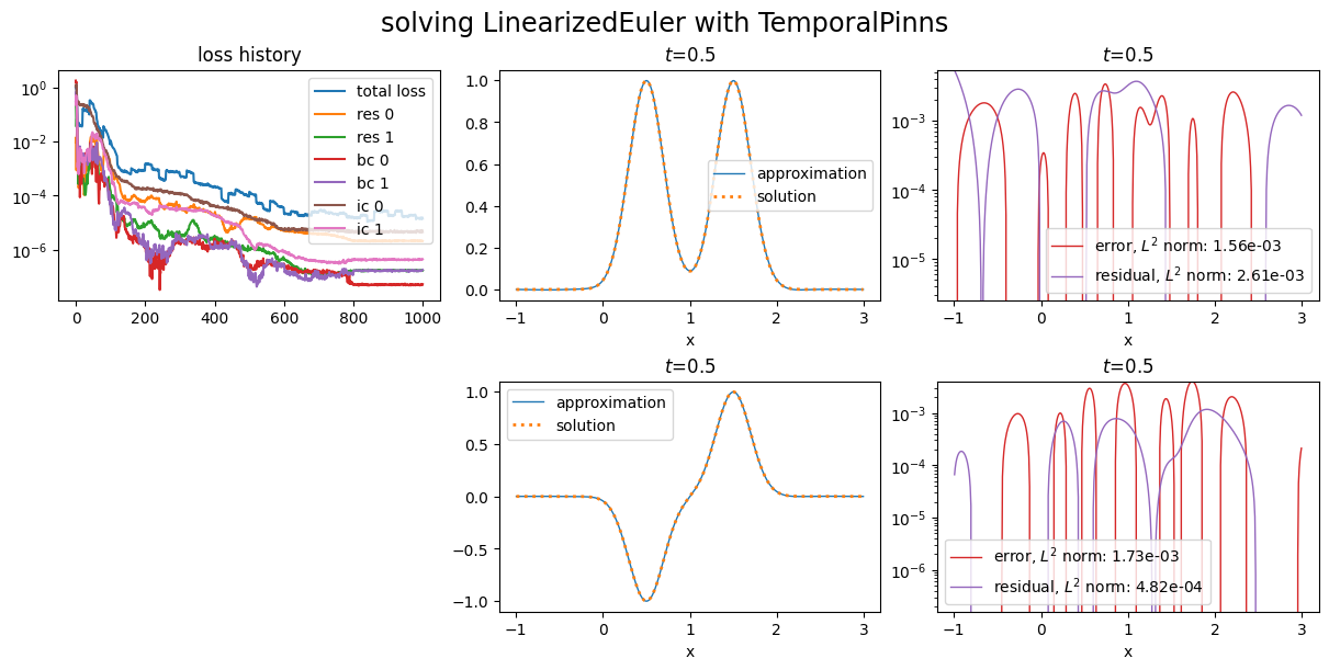
Let us try to improve this by setting \(w_{\text{ic}}\) to 1000:

space2 = NNxtSpace(2, 0, GenericMLP, domain_x, sampler, layer_sizes=[64])
pde2 = LinearizedEuler(space2, initial_solution)

pinn2 = TemporalPinns(
    pde2,
    bc_type="weak",
    ic_type="weak",
    ic_weight=1000.,
    one_loss_by_equation=True,
    optimizers="ssbfgs"
)

pinn2.solve(epochs=1000, n_collocation=3000)

Training: 100%|||||||||||||||| 1000/1000[00:19<00:00] , loss: 3.1e+02 -> 1.7e-03

plot_abstract_approx_spaces(
    pinn2.space,
    domain_x,
    domain_mu,
    domain_t,
    loss=pinn2.losses,
    residual=pde2,
    solution=exact_solution,
    error=exact_solution,
    title="solving LinearizedEuler with TemporalPinns",
)

plt.show()

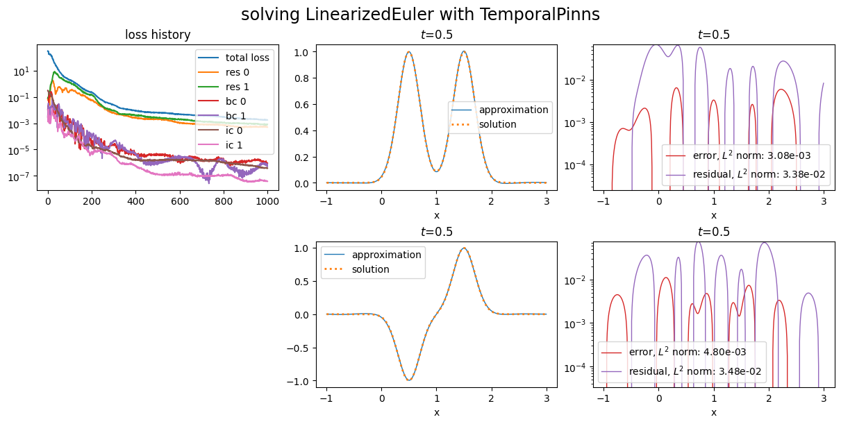
Notice the losses corresponding to initial conditions.

Now, let us give more weight to the first equation of the residual by setting \(w_{\text{in},0}=1\) with optional argument in_weights:

space3 = NNxtSpace(2, 0, GenericMLP, domain_x, sampler, layer_sizes=[64])
pde3 = LinearizedEuler(space3, initial_solution)

pinn3 = TemporalPinns(
    pde3,
    bc_type="weak",
    ic_type="weak",
    in_weights=[1000., 1.],
    one_loss_by_equation=True,
    optimizers="ssbfgs"
)

pinn3.solve(epochs=1000, n_collocation=3000)

Training: 100%|||||||||||||||| 1000/1000[00:17<00:00] , loss: 1.2e+01 -> 2.9e-04

plot_abstract_approx_spaces(
    pinn3.space,
    domain_x,
    domain_mu,
    domain_t,
    loss=pinn3.losses,
    residual=pde3,
    solution=exact_solution,
    error=exact_solution,
    title="solving LinearizedEuler with TemporalPinns",
)

plt.show()

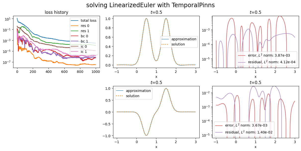
See loss histories corresponding to first and second equations.

In short:

• in_weight: modifies \(w_{\text{in}}\) the loss of all equations of the residual

• in_weights: modifies the \(w_{\text{in}, i}\)s, the losses for each equation of the residual

• bc_weight: modifies \(w_{\text{bc}}\) the loss of all equations of the boundary conditions

• bc_weights: modifies the \(w_{\text{bc}, j}\)s, the losses for each equation of the boundary conditions

• ic_weight: modifies \(w_{\text{ic}}\) the loss of all equations of the initial conditions

• ic_weights: modifies the \(w_{\text{ic}, k}\)s, the losses for each equation of the initial conditions

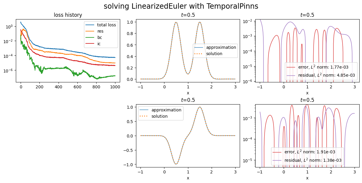
One can also simplify the plot showing the losses histories:

import matplotlib.pyplot as plt
from scimba_torch.plots.plots_nd import plot_abstract_approx_spaces

plot_abstract_approx_spaces(
    pinn.space,
    domain_x,
    domain_mu,
    domain_t,
    loss=pinn.losses,
    residual=pde,
    solution=exact_solution,
    error=exact_solution,
    title="solving LinearizedEuler with TemporalPinns",
    loss_groups=["res", "bc", "ic",],
)

plt.show()

Custom loss functions

One can also define custom loss function and use it in PINNs.

Let us define a PINN for our problem that uses Mean Absolute Error (L1) losses for the first equations of residual, boundary and initial conditions and MSE loss for the other one.

To this end, one should create an instance of the GenericLosses class with initialization argument being a list of triples as (label, evaluation function, weight):

from scimba_torch.optimizers.losses import GenericLosses

losses = GenericLosses(
    [
        ("res 0", torch.nn.L1Loss(), 1.0),
        ("res 1", torch.nn.MSELoss(), 1.0),
        ("bc 0", torch.nn.L1Loss(), 10.0),
        ("bc 1", torch.nn.MSELoss(), 10.0),
        ("ic 0", torch.nn.L1Loss(), 10.0),
        ("ic 1", torch.nn.MSELoss(), 10.0),
    ],
)

The order of the losses in the list matter, and the weights override the default weights.

space4 = NNxtSpace(2, 0, GenericMLP, domain_x, sampler, layer_sizes=[64])
pde4 = LinearizedEuler(space4, initial_solution)

pinn4 = TemporalPinns(
    pde4,
    bc_type="weak",
    ic_type="weak",
    losses=losses,
    optimizers="ssbfgs"
)

pinn4.solve(epochs=1000, n_collocation=3000)

Training: 100%|||||||||||||||| 1000/1000[00:17<00:00] , loss: 7.8e+00 -> 1.4e-02

plot_abstract_approx_spaces(
    pinn4.space,
    domain_x,
    domain_mu,
    domain_t,
    loss=pinn4.losses,
    residual=pde4,
    solution=exact_solution,
    error=exact_solution,
    title="solving LinearizedEuler with TemporalPinns",
)

plt.show()

Automatic weights update

Scimba implement the so called learning rate annealing. User can specify the principal weights, the learning rate annealing factor and the number of epochs between two updates:

losses = GenericLosses(
    [
        ("res 0", torch.nn.MSELoss(), 1.0),
        ("res 1", torch.nn.MSELoss(), 1.0),
        ("bc 0", torch.nn.MSELoss(), 10.0),
        ("bc 1", torch.nn.MSELoss(), 10.0),
        ("ic 0", torch.nn.MSELoss(), 10.0),
        ("ic 1", torch.nn.MSELoss(), 10.0),
    ],
    adaptive_weights="annealing",
    principal_weights="res 0", # default: the first loss in the list
    alpha_lr_annealing=0.999, # default: 0.9
    epochs_adapt=20, # default: 10
)

torch.manual_seed(0)

space5 = NNxtSpace(2, 0, GenericMLP, domain_x, sampler, layer_sizes=[64])
pde5 = LinearizedEuler(space5, initial_solution)

pinn5 = TemporalPinns(
    pde5,
    bc_type="weak",
    ic_type="weak",
    losses=losses,
    optimizers="ssbfgs"
)

pinn5.solve(epochs=1000, n_collocation=3000)

Training: 100%|||||||||||||||| 1000/1000[00:24<00:00] , loss: 9.7e-01 -> 1.0e-05

plot_abstract_approx_spaces(
    pinn5.space,
    domain_x,
    domain_mu,
    domain_t,
    loss=pinn5.losses,
    residual=pde5,
    solution=exact_solution,
    error=exact_solution,
    title="solving LinearizedEuler with TemporalPinns",
)

plt.show()

The losses argument can not be used with PINNs using natural gradient.

Data loss

Scimba offers the possibility to use, in addition to the residual losses, losses based on data. Let us first generate some data from the exact solution. Of course in the real life one does not have the exact solution and knows the data from another source.

n_samples_per_dim = 40
box = [(0., 0.5), (-1., 3.)]
linspaces = [torch.linspace(b[0], b[1], n_samples_per_dim) for b in box]
meshgrid = torch.meshgrid(*linspaces, indexing='xy')
mesh = torch.stack(meshgrid, axis=-1).reshape((n_samples_per_dim**2, 2))

t, x, mu = mesh[:, :1], mesh[:, 1:2], mesh[:, 2:]
y = exact_solution(LabelTensor(t), LabelTensor(x), LabelTensor(mu))

We now create the loss:

from scimba_torch.optimizers.losses import DataLoss

dloss = DataLoss((t, x, mu), y, torch.nn.MSELoss())

and the PINN to use it. One can instantiate a PINN with a list of data losses and a list of corresponding weights (optional argument dl_weights):

space6 = NNxtSpace(2, 0, GenericMLP, domain_x, sampler, layer_sizes=[64])
pde6 = LinearizedEuler(space6, initial_solution)

pinn6 = TemporalPinns(
    pde6,
    bc_type="weak",
    ic_type="weak",
    one_loss_by_equation=True,
    data_losses=[dloss],
    dl_weights=[10.0],
    optimizers="ssbfgs"
)

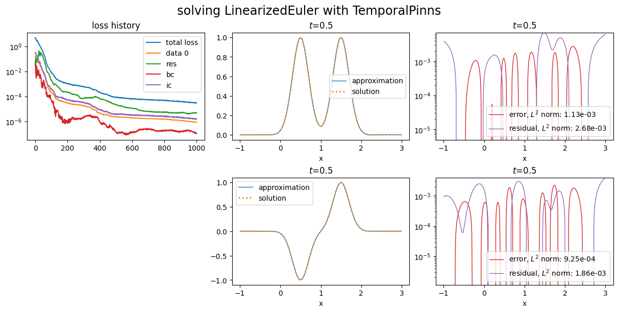
pinn6.solve(epochs=1000, n_collocation=3000)

Training: 100%|||||||||||||||| 1000/1000[00:16<00:00] , loss: 4.9e+00 -> 3.0e-05

plot_abstract_approx_spaces(
    pinn6.space,
    domain_x,
    domain_mu,
    domain_t,
    loss=pinn6.losses,
    residual=pde6,
    solution=exact_solution,
    error=exact_solution,
    title="solving LinearizedEuler with TemporalPinns",
    loss_groups=["res", "bc", "ic",],
)

plt.show()

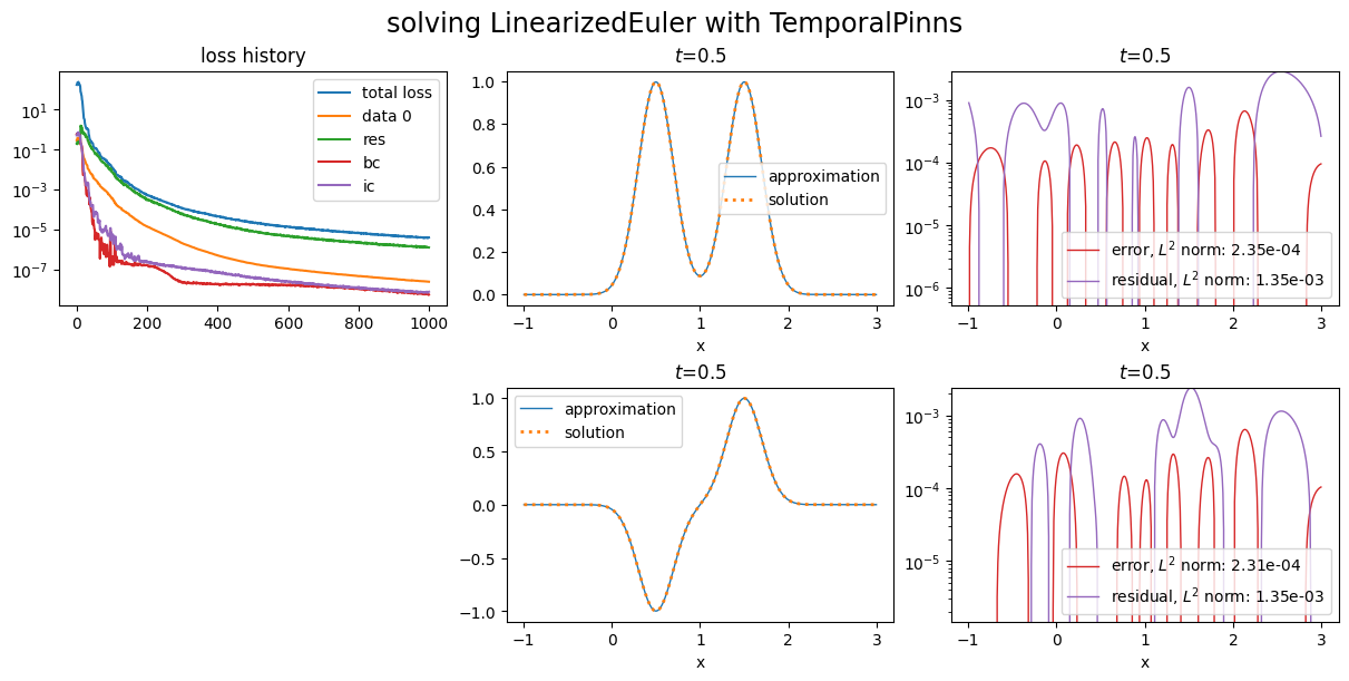
Data losses work with natural gradient PINNs:

from scimba_torch.numerical_solvers.temporal_pde.pinns import NaturalGradientTemporalPinns

space7 = NNxtSpace(2, 0, GenericMLP, domain_x, sampler, layer_sizes=[64])
pde7 = LinearizedEuler(space7, initial_solution)

pinn7 = NaturalGradientTemporalPinns(
    pde7,
    bc_type="weak",
    ic_type="weak",
    one_loss_by_equation=True,
    bc_weight =30.,
    ic_weight=300.,
    data_losses=[dloss],
    dl_weights=[10.0],
)

pinn7.solve(epochs=1000, n_collocation=3000)

Training: 100%|||||||||||||||| 1000/1000[01:36<00:00] , loss: 1.7e+02 -> 3.7e-06

plot_abstract_approx_spaces(
    pinn7.space,
    domain_x,
    domain_mu,
    domain_t,
    loss=pinn7.losses,
    residual=pde7,
    solution=exact_solution,
    error=exact_solution,
    title="solving LinearizedEuler with TemporalPinns",
    loss_groups=["res", "bc", "ic",],
)

plt.show()