Defining a physical model

This tutorial will present the main steps to implement the modelisation of a physical problem involving Partial Differential Equation (PDE) in scimba_jax, for 4 kinds of problems:

• 1-dimensional unknown function of space in homogeneous medium

• 1-dimensional unknown function of time and space in homogeneous medium

• 2-dimensional unknown function of time and space in homogeneous medium

• 1-dimensional unknown function of space in non-homogeneous medium

1-dimensional unknown function of space in homogeneous medium

In this first section, we will implement a 2D Laplacian with Dirichlet boundary conditions in an homogenous medium.

We consider the equation:

\[- \mu\Delta u = 2(2\mu\pi)^2 \sin(2\pi x) \sin(2\pi y)\]

on \((x,y) \in \Omega := [-1, 1]\times[-1, 1]\) with parameter \(\mu\in[1,2]\) subject to the Dirichlet condition:

\[u = 0\]

on \(\partial\Omega\).

The strong form of this problem will be implemented as a class, and an instance of this class will serve numerical approximation of the solution with a PINN.

Remark: the strong form of this problem is already implemented in the class ParametricLaplacianDirichletND and can be directly instantiated by users with:

import jax
import jax.numpy as jnp

def f_rhs(xy: jnp.ndarray, mu: jnp.ndarray) -> jnp.ndarray:
    x, y = xy[..., 0:1], xy[..., 1:2]
    return 2 * (mu[...,0:1] * jnp.pi)**2 * jnp.sin(jnp.pi * x) * jnp.sin(jnp.pi * y)

from scimba_jax.physical_models.elliptic_pde.laplacians import ParametricLaplacianDirichletND

try:
    model = ParametricLaplacianDirichletND(omega, f_rhs, bc="weak")  # noqa: F821
except Exception:
    pass

where omega is the geometric domain \(\Omega\), f_rhs is the right hand side of the residual, bc="weak" means that boundary conditions is handled weakly; see the complete example about Scimba basics.

The rest of this section describes the implementation of this class in a pedagogical aim.

Let us first define domains and samplers for this problem (see the tutorial on domains and samplers).

from scimba_jax.domains.meshless_domains.domains_2d import Square2D
from scimba_jax.nonlinear_approximation.integration.monte_carlo import (
    DomainSampler,
    TensorizedSampler,
)
from scimba_jax.nonlinear_approximation.integration.monte_carlo_parameters import (
    UniformParametricSampler,
)

domain_x = Square2D([(-1.0, 1.0), (-1.0, 1.0)], is_main_domain=True)
domain_mu = [(1., 2.)]
sampler = TensorizedSampler(
    [DomainSampler(domain_x), UniformParametricSampler(domain_mu)], bc=True
)

In scimba_jax, a problem is modeled with a dictionary of residuals; a residual is modeled by a functional operator that applies to the variable(s) \(u\) of the problem, and a right-hand side. We first introduce how we manipulate variables in scimba_jax.

Variables and Operators

In the PINN’s approach, an approximation of the solution \(u^*\) of a problem is sought in so called approximation space, that is a finite dimensional parameterized space of surrogate functions \(u_\theta\) that are Neural Networks (NN) with weights \(\theta\). An approximation is found by tuning the weights \(\theta\) to minimize the residuals:

\[\mathcal{R}_i(u_\theta) = f_i \text{ for }i=1,\ldots\]

where the \(\mathcal{R}_i\) are functional operators.

Implementing a residual in scimba_jax means implementing such a functional operator \(\mathcal{R}_i\).

For a parametric stationary problem, such a variable is a callable object like:

WEIGHTS_TYPE = any
def u_theta(theta: WEIGHTS_TYPE, xy: jnp.ndarray, mu: jnp.ndarray) -> jnp.ndarray:
    pass

Let us implement the left-hand side of a Laplacian residual \(\mathcal{R}\) such that for any \(u\):

\[\mathcal{R}(u): {\bf x}, \mu \mapsto - \mu\Delta u({\bf x}, \mu)\]

from typing import Callable

def LaplacianResidualOperator(var: Callable) -> Callable:
    #hessian of var
    hessian = jax.hessian(var, argnums=1) # hessian is a function
    #trace of hessian of var
    trace = lambda *args: jnp.trace(hessian(*args), axis1=-2, axis2=-1) # trace is a function
    #parametric laplacian operator
    return lambda theta, xy, mu: -mu*trace(theta, xy, mu)

Since we know the analytic expression of the solution of the problem, we can verify soundness of our implementation by defining the variable \(u^*\):

def analytic_solution(xy: jnp.ndarray, mu: jnp.ndarray) -> jnp.ndarray:
    x, y = xy[..., 0:1], xy[..., 1:2]
    return mu * jnp.sin(jnp.pi * x) * jnp.sin(jnp.pi * y)

def u_star(theta: WEIGHTS_TYPE, xy: jnp.ndarray, mu: jnp.ndarray) -> jnp.ndarray:
    return analytic_solution(xy, mu)

R_u_star = LaplacianResidualOperator(u_star)

On any point of the geometric domain, \(\mathcal{R}(u^*)\) and \(f\) must match:

N_COLLOC = 1000

import jax
key = jax.random.PRNGKey(0) #initialize the random generator
key, sample_dict = sampler.sample(key)
xy, mu = sample_dict["interior"]

batched_f_rhs = jax.vmap(f_rhs, in_axes=(0, 0))
batched_R_u_star = jax.vmap(R_u_star, in_axes=(None, 0, 0))

assert jnp.allclose( batched_f_rhs(xy, mu), batched_R_u_star(None, xy, mu) )

scimba_jax offers to simplify this implementation by providing special classes to manipulate variables: the ParamFunction class and its subclasses:

• ParamScalarFunction for scalar variables (most cases),

• ParamFieldFunction for field variables (for instance gradients of scalar variables),

• ParamVecFunction for vector variables,

• ParamMatrixFunction mostly used internally.

ParamFunction instances are callable objects, but offer more functionalities. For instance, our functional operator for the Laplacian residual could be rewritten:

from scimba_jax.nonlinear_approximation.model_class.funcparam_scalar import ParamScalarFunction

def LaplacianResidualOperator(var: ParamScalarFunction) -> ParamScalarFunction:
    lap = var.laplacian_x() # laplacian w.r.t x is implemented for ParamScalarFunctions
    return -lap * (lambda x, mu: mu) # scalar multiplication is overloaded for ParamScalarFunctions and regular callable objects

In order to test it, we create a ParamScalarFunction instance that encapsulates u_star (this deserves a pedagogical aim; in practice, users don’t have to create ParamFunctions on their own):

u_star_p = ParamScalarFunction(
    {"x":2, "mu":1}, # a dictionary symbol: dimension
    u_star, # the variable
    "x_mu", # the ordering of symbols in the call
)

Then apply the operator and verify:

R_u_star = LaplacianResidualOperator(u_star_p)
batched_R_u_star = jax.vmap(R_u_star, in_axes=(None, 0, 0))

assert jnp.allclose( batched_f_rhs(xy, mu), batched_R_u_star(None, xy, mu) )

The functional operator will now be encapsulated in a residual.

Residuals

There are 4 types of residuals in scimba_jax, implemented by 4 classes:

• InteriorResidual models residuals of the interior of the geometric domain,

• BoundaryResidual models boundary conditions,

• InitialResidual models initial conditions,

• DataResidual allows to implement data losses.

Let us implement a class for the parametric Laplacian operator as a subclass of InteriorResidual. Such a subclass must implement a method construct_residual which construct the left-hand side of the residual for a list of variables; here, this falls back to applying the Laplasian operator.

from scimba_jax.domains.meshless_domains.base import VolumetricDomain
from scimba_jax.physical_models.abstract_residuals import InteriorResidual

class ParametricLaplacianResidual(InteriorResidual):
    def __init__(
        self,
        domain: VolumetricDomain,
        f_rhs: Callable | None = None,
    ):
        super().__init__(domain=domain, size=1, model_type="x_mu", f_rhs=f_rhs)

    def construct_residual(self, *vars: ParamScalarFunction) -> ParamScalarFunction:
        return LaplacianResidualOperator(vars[0])

Initializing the InteriorResidual part requires:

• domain: the geometric domain, a scimba_jax instance of VolumetricDomain,

• size: the size of the operator (i.e. the dimension of the target space of \(\mathcal{R}(u)\)),

• model_type: a str describing the input arguments of the variables and their order in a call,

• f_rhs: the right-hand side of the residual (None holds for the identically zero function),

• for time-dependent, the time domain (as explained in next parts).

laplacian_residual = ParametricLaplacianResidual(domain_x, f_rhs)

R_u_star = laplacian_residual.construct_residual(u_star_p)
batched_R_u_star = jax.vmap(R_u_star, in_axes=(None, 0, 0))

assert jnp.allclose( batched_f_rhs(xy, mu), batched_R_u_star(None, xy, mu) )

Remark: When implementing the construct_residual method of a residual class corresponding to a functional operator \(\mathcal{R}\), it is important to keep in mind that:

• construct_residual takes in input a ParamFunc and returns a ParamFunc; it does not evaluate the residual;

• the output of construct_residual will be vmapped to apply to batches of vectors hence you do not have to worry about batches;

• construct_residual is applyied once before the training; as a consequence it might be a wrong choice to search efficiency at the expense of readability.

As a second example, we implement a subclass of BoundaryResidual for the Dirichlet residual defined as:

\[\mathcal{B}(u) = f\]

where the operator \(\mathcal{B}\) is identity: \(\mathcal{B}(u): ({\bf x}, \mu) \mapsto u({\bf x}, \mu)\).

Because the boundaries of a geometric domain can be composite, a BoundaryResidual instance is attached to a dictionary of instances of SurfacicDomain, the class modeling domains of dimension \(d'<d\) embedded in \(\mathbb{R}^d\):

from scimba_jax.domains.meshless_domains.base import SurfacicDomain
from scimba_jax.physical_models.abstract_residuals import BoundaryResidual

class DirichletResidual(BoundaryResidual):
    def __init__(
        self,
        domain: dict[str, SurfacicDomain],
        size: int = 1,
        model_type: str = "x_mu",
        f_rhs: Callable | None = None,
        time_domain: tuple[float, ...] | None = None,
    ):
        super().__init__(
            domain=domain,
            size=size,
            model_type=model_type,
            f_rhs=f_rhs,
            time_domain=time_domain,
        )

    def construct_residual(self, *vars):
        # Here assume that variables are functions of normals
        rho = vars[0]
        return rho

Notice that althought the model type here is "x_mu", the right-hand side, if provided, is required to depend explicitly on the normals, as in:

def f_bc_rhs(xy: jnp.ndarray, n: jnp.ndarray, mu: jnp.ndarray) -> jnp.ndarray:
    x = xy[..., 0:1]
    return jnp.zeros_like(x)

and it is assumed in the method construct_residual that input variables depend also on the normals:

def u_star_with_normals(theta: WEIGHTS_TYPE, xy: jnp.ndarray, n: jnp.ndarray, mu: jnp.ndarray) -> jnp.ndarray:
    return analytic_solution(xy, mu)

u_star_wn = ParamScalarFunction(
    {"x":2, "n":2, "mu":1}, # a dictionary symbol: dimension
    u_star_with_normals, # the variable
    "x_n_mu", # the ordering of symbols in the call
)

Remark: variables with normals as argument are automatically created in instances of BoundaryResidual.

By default, all the boundary elements of a VolumetricDomain which is a main domain are grouped in a dictionary; this dictionary has label "boundary":

boundaries_dict_of_dict = domain_x.get_all_boundaries()
#by default, this returns a dictionary with a unique entry with label "boundary"
#which is a dictionary
print(boundaries_dict_of_dict)

dirichlet_residual = DirichletResidual(boundaries_dict_of_dict["boundary"], 1, "x_mu", f_bc_rhs, None)

B_u_star = dirichlet_residual.construct_residual(u_star_wn)
batched_R_u_star = jax.vmap(B_u_star, in_axes=(None, 0, 0, 0))
batched_f_bc_rhs = jax.vmap(f_bc_rhs, in_axes=(0, 0, 0))

xy, n, mu = sample_dict["boundary"]
assert jnp.allclose( batched_f_bc_rhs(xy, n, mu), batched_R_u_star(None, xy, n, mu) )

{'boundary': {'bc south': SurfacicDomain with label "bc south" of type Segment2D, 'bc east': SurfacicDomain with label "bc east" of type Segment2D, 'bc north': SurfacicDomain with label "bc north" of type Segment2D, 'bc west': SurfacicDomain with label "bc west" of type Segment2D}}

InteriorResidual, BoundaryResidual and InitialResidual are all subclasses of PhysicalResidual.

Physical models

We are ready implement the class ParametricLaplacianDirichletND that models the condidered problem. It will inherit from the abstract class AbstractPhysicalModel of which a simplified version is reproduced below.

A physical model in scimba_jax is a dictionary of PhysicalResidual instances (and possibly a dictionary of DataResidual instances) attached to geometric and temporal domains:

import warnings
from abc import ABC
from scimba_jax.physical_models.abstract_residuals import DataResidual, PhysicalResidual

PHYSICAL_RESIDUALS_TYPE = dict[str, PhysicalResidual]
DATA_RESIDUALS_TYPE = dict[str, DataResidual]

class SimplifiedAbstractPhysicalModel(ABC):
    main_domain: VolumetricDomain
    time_domain: tuple[float, ...]
    dim: int
    boundaries: dict[str, dict[str, SurfacicDomain]]
    physical_residuals: PHYSICAL_RESIDUALS_TYPE
    data_residuals: DATA_RESIDUALS_TYPE

    def __init__(
        self,
        main_domain: VolumetricDomain,
        time_domain: tuple[float, float] | None = None,
    ):
        self.main_domain = main_domain
        self.time_domain = tuple() if time_domain is None else time_domain
        self.dim = self.main_domain.dim + int(time_domain is None)

        assert self.main_domain.is_main_domain
        try:
            self.boundaries = self.main_domain.get_all_boundaries()
        except NotImplementedError:
            self.boundaries = {group: {} for group in self.main_domain.boundaries}

        self.physical_residuals = {}
        self.data_residuals = {}

    def get_physical_residuals(self) -> PHYSICAL_RESIDUALS_TYPE:
        return self.physical_residuals

    def get_data_residuals(self) -> DATA_RESIDUALS_TYPE:
        return self.data_residuals

    # user can add data_residuals later
    def add_data_residual(self, label: str, residual: DataResidual):
        if label in self.data_residuals:
            warnings.warn("replacing data residual %s" % label, RuntimeWarning)
        self.data_residuals[label] = residual

Notice the automatic construction of the dictionary of dictionaries of boundary elements.

Here comes the class ParametricLaplacianDirichletND which gathers the interior and boundary residuals in the dictionary of physical residuals:

from scimba_jax.physical_models.abstract_physical_model import AbstractPhysicalModel

class ParametricLaplacianDirichletND(AbstractPhysicalModel):
    """A n D laplacian equation with one parameter."""

    def __init__(
        self,
        main_domain: VolumetricDomain,
        f_rhs: Callable | None = None,
        bc: str = "weak",
        f_bc_rhs: Callable | None = None,
    ):
        super().__init__(main_domain=main_domain)
        self.physical_residuals: PHYSICAL_RESIDUALS_TYPE = {
            self.main_domain.get_label(): ParametricLaplacianResidual(
                domain=main_domain,
                f_rhs=f_rhs,
            ),
        }

        if bc == "weak":
            for boundary in self.boundaries:
                self.physical_residuals[boundary] = DirichletResidual(
                    domain=self.boundaries[boundary],
                    model_type="x_mu",
                    f_rhs=f_bc_rhs,
                )

The boundary residual is created for all dictionaries of boundary elements.

Let us finally instantiate our model:

model = ParametricLaplacianDirichletND(domain_x, f_rhs, bc="weak")

Define and train a PINN for our physical model:

To finish with, we define and train a PINN to approximate the solution of the considered problem:

import matplotlib.pyplot as plt

from scimba_jax.nonlinear_approximation.networks.mlp import MLP
from scimba_jax.nonlinear_approximation.approximation_spaces.approximation_spaces import (
    ApproximationSpace,
)
from scimba_jax.nonlinear_approximation.numerical_solvers.projectors import Projector
from scimba_jax.plots.plots_nd import plot_abstract_approx_space

key = jax.random.PRNGKey(0) #initialize the random generator

nn = MLP(in_size=3, out_size=1, hidden_sizes=[16, 16, 16], key=key)
space = ApproximationSpace(
    {"x": 2, "mu": 1},       # x has dim 2, mu has dim 1
    [(nn, "scalar", None)],  # nn models a scalar function u
    model_type="x_mu",       # u depends of x and mu
)

The ApproximationSpace object automatically generates the variables of the problem.

pinn = Projector(model, space, sampler, matrix_regularization=1e-5)

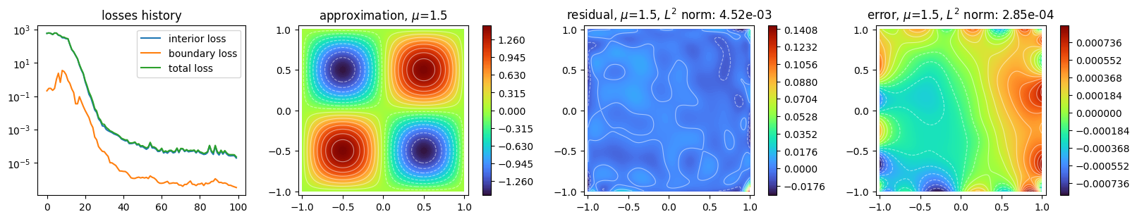
key, pinn = pinn.project(key, space, 100, 1000)

plot_abstract_approx_space(
    pinn.space,  # the approximation space
    domain_x,  # the spatial domain
    domain_mu,  # the parameter's domain
    loss=pinn.losses,  # for plot of the loss: the losses
    residual=pinn.model,  # for plot of the residual: the pde
    error=analytic_solution,  # for plot of the error with respect to a func: the func
    draw_contours=True,
    n_drawn_contours=20,
)
plt.show()

Training: 100%|||||||||||||||||| 100/100[00:03<00:00] , loss: 6.3e+02 -> 2.2e-05

1-dimensional unknown function of time and space in homogeneous medium

We consider a time-dependant 1D heat equation in an homogenous medium:

\[\frac{\partial}{\partial t} u - \Delta u = 0\]

on \(x \in \Omega := [0, 1]\) subject to the Dirichlet condition:

\[u = 0\]

on \(\partial\Omega\), and the initial condition:

\[u(0, x) = \sin(\pi x)\]

The strong form of this problem will be implemented as a class of which an instance will be used for solving with a PINN.

Remark: the strong form of this problem is already implemented in the class HeatND, see the complete example about Scimba basics.

The rest of this section describes the implementation of this class in a pedagogical aim.

Let us first define domains and samplers for this problem (see the tutorial on domains and samplers).

from scimba_jax.domains.meshless_domains.domains_1d import Segment1D
from scimba_jax.nonlinear_approximation.integration.monte_carlo_time import (
    UniformTimeSampler,
)

domain_t = (0.0, 1.0)
domain_x = Segment1D((0.0, 1.0), is_main_domain=True)

sampler = TensorizedSampler(
    [
        UniformTimeSampler(domain_t),
        DomainSampler(domain_x),
    ],
    model_type="t_x",
    bc=True,
    ic=True,
)

The analytic expression of the solution and the right-hand sides of the interior residual and the boundary conditions are time-dependent:

def analytic_solution(t: jnp.ndarray, x: jnp.ndarray):
    return jnp.exp(-(t * jnp.pi**2)) * jnp.sin(jnp.pi * x)

def f_rhs(t: jnp.ndarray, x: jnp.ndarray) -> jnp.ndarray:
    return jnp.zeros_like(x)

def f_bc_rhs(t: jnp.ndarray, x: jnp.ndarray, n: jnp.ndarray) -> jnp.ndarray:
    return jnp.zeros_like(x)

while the initial condition is not:

def f_init(x: jnp.ndarray):
    t = jnp.zeros_like(x)
    return analytic_solution(t, x)

Variables

Variables manipulated in time-dependent problems are callable objet with prototypes:

def u_theta(theta: WEIGHTS_TYPE, t: jnp.ndarray, x: jnp.ndarray) -> jnp.ndarray:
    pass

u_theta_p = ParamScalarFunction(
    {"t":1, "x":1}, # a dictionary symbol: dimension
    u_theta, # the variable
    "t_x", # the ordering of symbols in the call
)

def u_star(theta: WEIGHTS_TYPE, t: jnp.ndarray, x: jnp.ndarray) -> jnp.ndarray:
    return analytic_solution(t, x)

u_star_p = ParamScalarFunction(
    {"t":1, "x":1},
    u_star,
    "t_x",
)

Residuals

We will now implement the three residuals of our problem.

First the heat equation residual, which applies to the interior of the domain. Notice now the initialization of the InteriorResidual object with named argument time_domain; notice also the model_type="t_x":

class HeatResidual(InteriorResidual):
    def __init__(
        self,
        domain: VolumetricDomain,
        time_domain: tuple[float, float],
        f_rhs: Callable | None = None,
    ):
        super().__init__(
            domain=domain,
            size=1,
            model_type="t_x",
            f_rhs=f_rhs,
            time_domain=time_domain,
        )

    def construct_residual(self, *vars):
        rho = vars[0]
        assert isinstance(rho, ParamScalarFunction)
        lap = rho.laplacian_x()
        dt_rho = rho.d_t()
        return dt_rho - lap

We instantiate it and check soundness on the analytic solution:

heat_residual = HeatResidual(domain_x, domain_t, f_rhs)

R_u_star = heat_residual.construct_residual(u_star_p)

key, sample_dict = sampler.sample(key)
t, x = sample_dict["interior"]

batched_f_rhs = jax.vmap(f_rhs, in_axes=(0, 0))
batched_R_u_star = jax.vmap(R_u_star, in_axes=(None, 0, 0))

assert jnp.allclose( batched_f_rhs(t, x), batched_R_u_star(None, t, x) )

The class DirichletResidual is already defined above, and it remains to define a class for the initial condition that will inherit from InitialResidual:

from scimba_jax.physical_models.abstract_residuals import InitialResidual

class ProjectionResidual(InitialResidual):
    def __init__(
        self,
        domain: VolumetricDomain,
        time_domain: float | tuple[float] = (0.0,),
        size: int = 1,
        model_type: str = "t_x",
        f_rhs: Callable | None = None, # a function that does not depend on time
    ):
        super().__init__(
            domain=domain,
            time_domain=(
                (time_domain,) if isinstance(time_domain, float) else time_domain
            ),
            size=size,
            model_type=model_type,
            f_rhs=f_rhs,
        )

    def construct_residual(self, *vars):
        rho = vars[0]
        return rho.set_t_0(self.time_domain[0])

The set_t_0 method of a ParamScalarFunction fixes the value of \(t\); here construct_residual construct a ParamScalarFunction of type x from a ParamScalarFunction of type t_x:

initial_residual = ProjectionResidual(domain_x, domain_t[0], f_rhs=f_init)

I_u_star = initial_residual.construct_residual(u_star_p)
assert I_u_star.f_type == "x"

key, sample_dict = sampler.sample(key)
x, = sample_dict["ic interior"]

batched_f_init = jax.vmap(f_init, in_axes=(0))
batched_I_u_star = jax.vmap(I_u_star, in_axes=(None, 0))

assert jnp.allclose( batched_f_init(x), batched_I_u_star(None, x) )

Physical model:

As previously, we contruct a class to gather the three residuals in a dictionary:

class HeatND(AbstractPhysicalModel):
    def __init__(
        self,
        main_domain: VolumetricDomain,
        time_domain: tuple[float, float],
        f_rhs: Callable | None = None,
        bc: str = "weak",
        f_bc_rhs: Callable | None = None,
        ic: str = "weak",
        f_ic_rhs: Callable | None = None,
    ):
        super().__init__(main_domain=main_domain, time_domain=time_domain)
        self.physical_residuals: PHYSICAL_RESIDUALS_TYPE = {
            self.main_domain.get_label(): HeatResidual(
                domain=main_domain,
                time_domain=time_domain,
                f_rhs=f_rhs,
            ),
        }
        if bc == "weak":
            for boundary in self.boundaries:
                self.physical_residuals[boundary] = DirichletResidual(
                    domain=self.boundaries[boundary],
                    time_domain=time_domain,
                    model_type="t_x",
                    f_rhs=f_bc_rhs,
                )
        if ic == "weak":
            label = "ic " + self.main_domain.get_label()
            self.physical_residuals[label] = ProjectionResidual(
                domain=main_domain,
                time_domain=(self.time_domain[0],),
                model_type="t_x",
                f_rhs=f_ic_rhs,
            )

Let us finally instantiate our model:

model = HeatND(domain_x, domain_t, bc="weak", ic="weak", f_ic_rhs=f_init)

The right-hand sides for the interior and the boundary residual are zero functions.

Define and train a PINN for our physical model:

To finish with, we define and train a PINN to approximate the solution of the considered problem:

key = jax.random.PRNGKey(0)
nn = MLP(in_size=2, out_size=1, hidden_sizes=[16, 16], key=key)

space = ApproximationSpace(
    {"x": 2}, # t is implicitly of dim 1
    [(nn, "scalar", None)],
    model_type="t_x",
)

pinn = Projector(model, space, sampler)
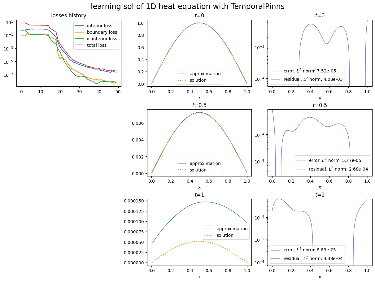
key, pinn = pinn.project(
    key, space, 50, 1000, 1000, 1000
)

plot_abstract_approx_space(
    pinn.space,
    domain_x,
    time_domain=domain_t,
    time_values=[0.0, .5, 1.],
    loss=pinn.losses,
    residual=pinn.model,
    solution=analytic_solution,
    error=analytic_solution,
    title="learning sol of 1D heat equation with TemporalPinns",
)

plt.show()

Training: 100%|||||||||||||||||||| 50/50[00:01<00:00] , loss: 6.5e+00 -> 3.4e-07

2-dimensional unknown function of time and space in homogeneous medium

We consider a time-dependant 1D problem with 2-dimensional unknown function \(u=(u_1, u_2)\) (which is called Linearized Euler problem):

\[\begin{split}\left\{\begin{array}{rl} \frac{\partial}{\partial t} u_1 - \frac{\partial}{\partial x} u_2 &= 0\\ \frac{\partial}{\partial t} u_2 - \frac{\partial}{\partial x} u_1 &= 0 \end{array}\right.\end{split}\]

on \(x \in \Omega := [0, 1]\) subject to the Dirichlet condition:

\[\begin{split}\left\{\begin{array}{rl} u_1 &= 0 \\ u_2 &= 0 \\ \end{array}\right.\end{split}\]

on \(\partial\Omega\), and the initial condition:

\[\begin{split}\left\{\begin{array}{rl} u_1(0, x) &= \frac{1}{4\pi D} \exp\left( -\frac{(x-1)^2}{4D} \right) \\ u_2(0, x) &= 0 \end{array}\right.\end{split}\]

where \(D = 0.02\).

We first define the domains and a sampler; once again, the parametric domain is empty.

t_min, t_max = 0.0, 0.5
domain_t = (t_min, t_max)
domain_x = Segment1D((-1.0, 3.0), is_main_domain=True)

sampler = TensorizedSampler(
    [
        UniformTimeSampler(domain_t),
        DomainSampler(domain_x),
    ],
    model_type="t_x",
    bc=True,
    ic=True,
)

Rather than seeing the residuals as systemes of two equations in two variables \(u_1\) and \(u_2\), we consider one vectorial variable \({\bf u}\) taking its values in \(\mathbb{R}^2\):

\[{\bf u}: x, \mu \mapsto \left(u_1(x, \mu), u_2(x, \mu)\right)\]

The considered problem has a solution with analytic expression:

def analytic_solution(t, x):
    D = 0.02
    coeff = 1 / (4 * jnp.pi * D) ** 0.5
    u1_plus_u2 = coeff * jnp.exp(-((x - t - 1) ** 2) / (4 * D))
    u1_minus_u2 = coeff * jnp.exp(-((x + t - 1) ** 2) / (4 * D))
    u1 = (u1_plus_u2 + u1_minus_u2) / 2
    u2 = (u1_plus_u2 - u1_minus_u2) / 2
    return jnp.concatenate((u1, u2), axis=-1)

which specializes in the initial solution:

def initial_solution(x):
    return analytic_solution(jnp.zeros_like(x), x)

This time, we will manipulate ParamVecFunction instances of size 2 like:

from scimba_jax.nonlinear_approximation.model_class.funcparam_vectorial import ParamVecFunction

def u_star(theta: WEIGHTS_TYPE, t: jnp.ndarray, x: jnp.ndarray) -> jnp.ndarray:
    return analytic_solution(t, x)

u_star_p = ParamVecFunction(
    2, #the out size
    {"t":1, "x":1}, #the in sizes
    u_star,
    "t_x",
)

Here is how one can implement the Linearized Euler residual:

class LinearizedEulerResidual(InteriorResidual):
    def __init__(
        self,
        domain: VolumetricDomain,
        time_domain: tuple[float, float],
        f_rhs: Callable | None = None,
    ):
        super().__init__(
            domain=domain,
            size=2,
            model_type="t_x",
            f_rhs=f_rhs,
            time_domain=time_domain,
        )

    def construct_residual(self, *vars):
        rho = vars[0]
        assert isinstance(rho, ParamVecFunction)
        dt_rho = rho.d_t()
        dx_rho = rho.partial_derivative_x(0)
        dx_rho = dx_rho.roll(1)
        return dt_rho + dx_rho

We instantiate it and check soundness on the analytic solution:

linearized_euler_residual = LinearizedEulerResidual(domain_x, domain_t)

R_u_star = linearized_euler_residual.construct_residual(u_star_p)

key, sample_dict = sampler.sample(key)
t, x = sample_dict["interior"]

batched_f_rhs = jax.vmap(f_rhs, in_axes=(0, 0))
batched_R_u_star = jax.vmap(R_u_star, in_axes=(None, 0, 0))

assert jnp.allclose( batched_f_rhs(t, x), batched_R_u_star(None, t, x) )

Let us implement Linearized Euler model as:

class LinearizedEuler(AbstractPhysicalModel):
    def __init__(
        self,
        main_domain: VolumetricDomain,
        time_domain: tuple[float, float],
        f_rhs: Callable | None = None,
        bc: str = "weak",
        f_bc_rhs: Callable | None = None,
        ic: str = "weak",
        f_ic_rhs: Callable | None = None,
    ):
        super().__init__(main_domain=main_domain, time_domain=time_domain)
        self.physical_residuals: PHYSICAL_RESIDUALS_TYPE = {
            self.main_domain.get_label(): LinearizedEulerResidual(
                domain=main_domain,
                time_domain=time_domain,
                f_rhs=f_rhs,
            ),
        }
        if bc == "weak":
            for boundary in self.boundaries:
                self.physical_residuals[boundary] = DirichletResidual(
                    domain=self.boundaries[boundary],
                    time_domain=time_domain,
                    size=2,
                    model_type="t_x",
                    f_rhs=f_bc_rhs,
                )
        if ic == "weak":
            label = "ic " + self.main_domain.get_label()
            self.physical_residuals[label] = ProjectionResidual(
                domain=main_domain,
                time_domain=(self.time_domain[0],),
                size=2,
                model_type="t_x",
                f_rhs=f_ic_rhs,
            )

and instantiate it:

model = LinearizedEuler(
    main_domain=domain_x, time_domain=domain_t, f_ic_rhs=initial_solution
)

Define and train a PINN for our physical model:

To finish with, we define and train a PINN to approximate the solution of the considered problem.

When creating the approximation space, we specify that the variable associated with the NN is a ParamVecFunction of size 2:

key = jax.random.PRNGKey(0)
nn = MLP(in_size=2, out_size=2, hidden_sizes=[32, 32], key=key)

space = ApproximationSpace(
    {"x": 1}, # t is implicitely of dim 1
    [(nn, "vec", 2)], # here we specify that the variable associated to nn is
    model_type="t_x"
)

pinn = Projector(model, space, sampler)

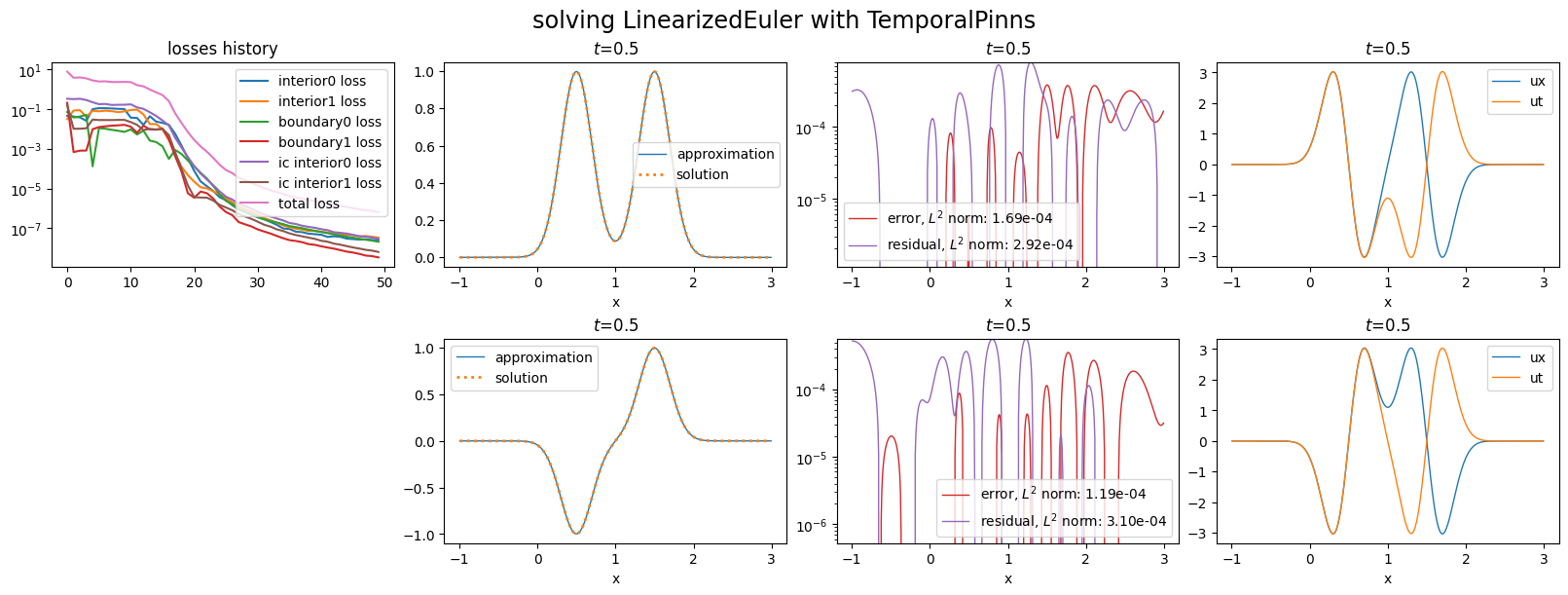
key, pinn = pinn.project(
    key, space, 50, 1000, 2000, 2000
)

plot_abstract_approx_space(
    pinn.space,
    domain_x,
    time_domain=domain_t,
    components=[0, 1],
    loss=pinn.losses,
    residual=pinn.model,
    solution=analytic_solution,
    error=analytic_solution,
    derivatives=["ux", "ut"],
    title="solving LinearizedEuler with TemporalPinns",
)

plt.show()

Training: 100%|||||||||||||||||||| 50/50[00:10<00:00] , loss: 3.9e+00 -> 6.4e-07

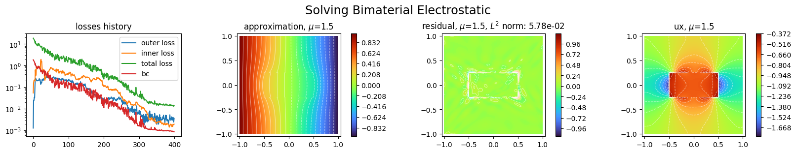
1-dimensional unknown function of space in non-homogeneous medium

We consider in this section a electrostatic problem which consist in solving a lagrangian on a domain composed of two nested rectangles: \(\Omega := [-1, 1]\times[-1, 1]\) and \(\Omega_{i} := [-1/2, 1/2]\times[-1/4, 1/4]\).

\(\Omega_{o} := \Omega \setminus \Omega_{i}\) and \(\Omega_{i}\) represent two different materials.

The problem is:

\[\begin{split}\left\{\begin{array}{rl} - \Delta u &= 0 \text{ on } \Omega_{o}\\ - 5\Delta u &= 0 \text{ on } \Omega_{i} \end{array}\right.\end{split}\]

with boundary conditions on \(\partial \Omega_{o}\):

\[\begin{split}\left\{\begin{array}{rl} \frac{\partial}{\partial y} u &= 0 \text{ on } y = -1\\ \frac{\partial}{\partial y} u &= 0 \text{ on } y = 1\\ u &= 1 \text{ on } x = -1\\ u &= -1 \text{ on } x = 1\\ \end{array}\right.\end{split}\]

with a discontinuity of \(\frac{\partial}{\partial x}u\) and \(\frac{\partial}{\partial y}u\) on \(\partial \Omega_{i}\):

\[\begin{split}\left\{\begin{array}{rl} \lim_{ (x,y) \rightarrow \partial \Omega_{i}, (x,y) \notin \Omega_{i}}\frac{\partial}{\partial y} u &= 3.3 \lim_{ (x,y) \rightarrow \partial \Omega_{i}, (x,y) \in \Omega_{i}}\frac{\partial}{\partial y} u \text{ on } y = +/- 1/4\\ \lim_{ (x,y) \rightarrow \partial \Omega_{i}, (x,y) \notin \Omega_{i}}\frac{\partial}{\partial x} u &= 3.3 \lim_{ (x,y) \rightarrow \partial \Omega_{i}, (x,y) \in \Omega_{i}}\frac{\partial}{\partial x} u \text{ on } x = +/- 1/2\\ \end{array}\right.\end{split}\]

Domains and samplers

We first define the geometric domains \(\Omega_{o}\) and \(\Omega_{i}\) as sub-domains of a scimba_jax domain representing \(\Omega\):

bounds_x = [(-1.0, 1.0), (-1.0, 1.0)]
bounds_ix = [(-0.5, 0.5), (-0.25, 0.25)]

omega = Square2D(bounds_x, is_main_domain=True, label_str="outer")
omega_i = Square2D(bounds_ix, is_main_domain=False, label_str="inner")

omega.add_subdomain(omega_i)

The boundaries elements of omega and omega are respectively called:

_ = tuple(print(bc.get_label()) for bc in omega.full_bc_domain())

bc south
bc east
bc north
bc west

_ = tuple(print(bc.get_label()) for bc in omega_i.full_bc_domain())

bc inner south
bc inner east
bc inner north
bc inner west

We group these boundaries element in a dictionary attached to omega:

omega.set_boundaries_dict(
    {
        "bc SN": ["bc south", "bc north"],
        "bc E": ["bc east"],
        "bc W": ["bc west"],
        "bc inner_SN": ["bc inner south", "bc inner north"],
        "bc inner_WE": ["bc inner west", "bc inner east"],
    }
)

and define a sampler:

sampler = TensorizedSampler(
    [DomainSampler(omega)], bc=True, model_type="x",
)

Let us try the sampler:

key = jax.random.PRNGKey(0)
key, dict_of_samples = sampler.sample(key, 1000)

def plot_dict_of_samples_2d(
    dict_of_samples: dict[str, tuple[jnp.ndarray, ...]],
    fig=None, index=111
):
    if fig is None:
        fig = plt.figure()
    axe=fig.add_subplot(index)
    for label in dict_of_samples:
        x, y = dict_of_samples[label][0][:,0], dict_of_samples[label][0][:,1]
        axe.scatter(x, y, s=2, label=label)
    axe.legend()
    axe.axis('equal')
    return fig

#dict_of_samples = dict_of_samples | sampler.bc_sample(key, 5000)

plot_dict_of_samples_2d(dict_of_samples)
plt.show()

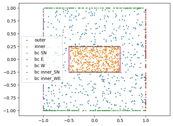
Notice that the samples labeled “outer” are points in \(\Omega_o\) and not in \(\Omega\).

To know more about scimba_jax domains, follow the tutorial on domains and samplers.

Neural Network and Unknown function

The main pittfall that one might face when approximating a solution of this problem with a neural network is the discontinuity of the unknown \(u\) at interface of \(\Omega_{o}\) and \(\Omega_{i}\).

To tackle it, we will approximate \(u\) with a function with 2 dimensional output, say

\[{\bf u}_{\theta} = \left( u^o_{\theta}, u^i_{\theta} \right)\]

where \(u^o_{\theta}\) approximates \(u\) on \(\Omega_o\) and \(u^i_{\theta}\) approximates \(u\) on \(\Omega_i\).

Let us create a approximation space:

key = jax.random.PRNGKey(0)

nn = MLP(in_size=2, out_size=2, hidden_sizes=[16, 16, 16], key=key)
space = ApproximationSpace({"x": 2}, [(nn, "vec", 2)], model_type="x")

Residuals

The interior residual becomes a system of equations:

\[\begin{split}\left\{\begin{array}{rl} - \Delta u^o_{\theta} &= 0 \text{ on } \Omega_{o}\\ - 5\Delta u^i_{\theta} &= 0 \text{ on } \Omega_{i} \end{array}\right.\end{split}\]

We define a dedicated residual class for this scaled Laplacian residual that will be instantiated two times, once for each equation:

class BiScaledLaplacian(InteriorResidual):
    def __init__(
        self,
        scale: float,
        component: int,
        domain: VolumetricDomain,
        f_rhs: Callable | None = None,
    ):
        super().__init__(domain=domain, size=1, model_type="x", f_rhs=f_rhs)
        self.scale = scale
        self.component = component

    def construct_residual(self, *vars):
        rho = vars[0]
        assert isinstance(rho, ParamVecFunction)
        # select component
        rho_c = rho.component(self.component)
        # compute laplacian
        lap_c = rho_c.laplacian_x()
        # scale by factor
        return -self.scale * lap_c

Boundary conditions rewrite:

\[\begin{split} \left\{\begin{array}{rl} \frac{\partial}{\partial y} u^o_{\theta} = 0 & \text{ on } y = +/- 1\\ u^o_{\theta} = 1 & \text{ on } x = -1\\ u^o_{\theta} = -1 & \text{ on } x = 1\\ \left\{\begin{array}{r} u^o_{\theta} = u^o_{\theta}\\ \frac{\partial}{\partial y} u^o_{\theta} = 3.3 \frac{\partial}{\partial y} u^i_{\theta}\\ \end{array}\right. & \text{ on } \{x,y \in \partial\Omega_{i} | y = +/- 1/4 \}\\ \left\{\begin{array}{r} u^o_{\theta} = u^o_{\theta}\\ \frac{\partial}{\partial x} u^o_{\theta} = 3.3 \frac{\partial}{\partial x} u^i_{\theta}\\ \end{array}\right. & \text{ on } \{x,y \in \partial\Omega_{i} | x = +/- 1/2 \}\\ \end{array}\right.\end{split}\]

The first equation is a Neumann condition while the second and the third are Dirichlet conditions.

We group the remaining ones in two systems of two equations.

The Neumann condition:

from scimba_jax.nonlinear_approximation.model_class.funcparam_field import ParamFieldFunction

class BiNeumannResidual(BoundaryResidual):
    def __init__(
        self,
        component: int,
        domain: dict[str, SurfacicDomain],
        f_rhs: Callable | None = None,
    ):
        super().__init__(
            domain=domain,
            size=1,
            model_type="x",
            f_rhs=f_rhs,
            time_domain=None,
        )
        self.component = component

    def construct_residual(self, *vars):
        rho = vars[0]
        assert isinstance(rho, ParamVecFunction)
        rho_index = rho.component(self.component)
        grad_x_rho = rho_index.gradient_x() # grad_x_rho is a ParamFieldFunction
        n_func = ParamFieldFunction(
            rho.dims,
            lambda *args: args[rho.argnums["n"]],
            rho.f_type,
        ) # n_func is a ParamFieldFunction that takes value "n", i.e. the normals
        grad_n_rho = grad_x_rho.dot(n_func) #dimensions match
        return grad_n_rho

The Dirichlet condition:

class BiDirichletResidual(BoundaryResidual):
    def __init__(
        self,
        component: int,
        domain: dict[str, SurfacicDomain],
        f_rhs: Callable | None = None,
    ):
        super().__init__(
            domain=domain,
            size=1,
            model_type="x",
            f_rhs=f_rhs,
            time_domain=None,
        )
        self.component = component

    def construct_residual(self, *vars):
        rho = vars[0]
        assert isinstance(rho, ParamVecFunction)
        rho_index = rho.component(self.component)
        return rho_index

And the interface condition:

class InterfaceResidual(BoundaryResidual):
    def __init__(
        self,
        factor: float,
        component: int,
        domain: dict[str, SurfacicDomain],
        f_rhs: Callable | None = None,
    ):
        super().__init__(domain=domain, size=2, model_type="x", f_rhs=f_rhs)

        self.factor = factor
        self.component = component

    def construct_residual(self, *vars):
        rho = vars[0]
        assert isinstance(rho, ParamVecFunction)
        # split outputs
        rho_i = rho.component(0)
        rho_o = rho.component(1)
        # compute partial derivative with respect to symbol
        rho_i_index = rho_i.partial_derivative_x(component_index=self.component)
        rho_o_index = rho_o.partial_derivative_x(component_index=self.component)
        # scale by factor
        equality = rho_i - rho_o
        discontinuity = rho_i_index - self.factor * rho_o_index
        return ParamVecFunction.cat([equality, discontinuity])

Physical model

We group right-hand sides of residuals in dictionaries:

f_rhs = {
    "inner": lambda *args: 0.0,
    "outer": lambda *args: 0.0,
}
f_bc_rhs = {
    "bc SN": lambda *args: 0.0,
    "bc E": lambda *args: -1.0,
    "bc W": lambda *args: 1.0,
    "bc inner_SN": lambda *args: 0.0,
    "bc inner_WE": lambda *args: 0.0,
}

And define the physical model corresponding to our bi-material electrostatic problem:

class BiMaterialElectrostatic(AbstractPhysicalModel):
    """BiMaterialElectrostatic model."""

    def __init__(self, main_domain, f_rhs, f_bc_rhs):
        super().__init__(main_domain=main_domain)

        self.e_r = 3.3
        # inner residuals
        self.physical_residuals = {
            "outer": BiScaledLaplacian(
                scale=1.0, component=0, domain=main_domain, f_rhs=f_rhs["outer"]
            ),
            "inner": BiScaledLaplacian(
                scale=5.0, component=1, domain=main_domain, f_rhs=f_rhs["inner"]
            ),
        }
        # boundary residuals
        self.physical_residuals["bc SN"] = BiNeumannResidual(
            component=0,
            domain=self.boundaries["bc SN"],
            f_rhs=f_bc_rhs["bc SN"],
        )
        self.physical_residuals["bc E"] = BiDirichletResidual(
            component=0,
            domain=self.boundaries["bc E"],
            f_rhs=f_bc_rhs["bc E"],
        )
        self.physical_residuals["bc W"] = BiDirichletResidual(
            component=0,
            domain=self.boundaries["bc W"],
            f_rhs=f_bc_rhs["bc W"],
        )
        self.physical_residuals["bc inner_SN"] = InterfaceResidual(
            factor=self.e_r,
            component=1,
            domain=self.boundaries["bc inner_SN"],
            f_rhs=f_bc_rhs["bc inner_SN"],
        )
        self.physical_residuals["bc inner_WE"] = InterfaceResidual(
            factor=self.e_r,
            component=0,
            domain=self.boundaries["bc inner_WE"],
            f_rhs=f_bc_rhs["bc inner_WE"],
        )

Let us instantiate it:

model = BiMaterialElectrostatic(omega, f_rhs, f_bc_rhs)

Define and train a PINN for our physical model:

To finish with, we define and train a PINN to approximate the solution of the considered problem.

N_EPOCHS = 400
N_COLLOC = 2000
N_BC_COLLOC = 6000

pinn = Projector(model, space, sampler, matrix_regularization=5e-4)

key, pinn = pinn.project(
    key, space, N_EPOCHS, N_COLLOC, N_BC_COLLOC
)

plot_abstract_approx_space(
    pinn.space,
    omega,
    domain_mu,
    loss=pinn.losses,
    residual=pinn.model,
    derivatives=["ux"],
    components=[{"outer": 0, "inner": 1}], # to assemble components in a single plot
    draw_contours=True,
    n_drawn_contours=20,
    title="Solving Bimaterial Electrostatic",
    loss_groups=["bc"], # to group losses corresponding to boundary conditions
)
plt.show()

Training: 100%|||||||||||||||||| 400/400[00:33<00:00] , loss: 1.7e+01 -> 1.3e-02