Domains and Samplers

ScimBa is designed to handle physical problems involving time, space, velocity, and parameters. Each of these variables is typically defined over its own domain. Since ScimBa employs a meshless approach for physical solution approximation, it requires defining appropriate samplers for each domain.

This tutorial covers:

• Geometric domains (volumetric and surfacic domains)

• Temporal and parametric domains with their samplers

• Kinetic domains and their corresponding samplers

• Tensorized samplers for composite domains

• Creating custom domains in scimba_jax

• generic (in dimension) domains

Currently, ScimBa supports only uniform samplers.

import jax
import jax.numpy as jnp
import scimba_jax

Geometric Domains and Samplers

Creating a Geometric Domain

Let us define a domain representing a segment of \(\mathbb{R}\):

from scimba_jax.domains.meshless_domains.domains_1d import Segment1D

segment = Segment1D((0., 1.), is_main_domain=True)
print(segment)

VolumetricDomain with label "interior" of type Segment1D main domain

segment is a VolumetricDomain, i.e. a domain with non-zero measure, and it is a main domain. This means it can be extended by adding mappings, holes, or subdomains.

In ScimBa, a physical problem must be attached to a VolumetricDomain object that is a main domain.

By default, a VolumetricDomain is labeled "interior". You can specify a label at instantiation:

segment = Segment1D((0., 1.), is_main_domain=True, label_str="seg", label_idx="1")
print(segment)

VolumetricDomain with label "seg 1" of type Segment1D main domain

Subdomains

Let us create a more complex domain, such as two nested rectangles with labels "outer" and "inner":

from scimba_jax.domains.meshless_domains.domains_2d import Square2D

bounds_o = [(-1.0, 1.0), (-1.0, 1.0)]
bounds_i = [(-0.7, 0.3), (-0.25, 0.25)]
big_square = Square2D(bounds_o, is_main_domain=True, label_str="outer")
small_square = Square2D(bounds_i, is_main_domain=False, label_str="inner")

big_square.add_subdomain(small_square)

print(big_square)
print("\n")
print(small_square)

VolumetricDomain with label "outer" of type Square2D main domain,
   - with subdomains: ["inner", ]


VolumetricDomain with label "inner" of type Square2D sub-domain

Samplers for Geometric Domains

ScimBa provides predefined uniform samplers for VolumetricDomains that are main domains:

from scimba_jax.nonlinear_approximation.integration.monte_carlo import DomainSampler

sampler = DomainSampler(big_square)

A sampler has a sample method to draw random points in the domain; it takes in input a random state and a number of points to sample and returns a new random state and a dictionary of samples:

key = jax.random.PRNGKey(0) #initialize the random generator

key, dict_of_samples = sampler.sample(key, 1000) #sample the domain

for label in dict_of_samples:
    print("label: %s, %d points" % (label, dict_of_samples[label][0].shape[0]))

label: outer, 500 points
label: inner, 500 points

Let us plot the samples:

import matplotlib.pyplot as plt

def plot_dict_of_samples_2d(
    dict_of_samples: dict[str, tuple[jnp.ndarray, ...]],
    fig=None, index=111
):
    if fig is None:
        fig = plt.figure()
    axe=fig.add_subplot(index)
    for label in dict_of_samples:
        x, y = dict_of_samples[label][0][:,0], dict_of_samples[label][0][:,1]
        axe.scatter(x, y, s=2, label=label)
    axe.legend()
    axe.axis('equal')
    return fig


plot_dict_of_samples_2d(dict_of_samples)
plt.show()

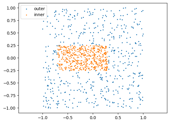
It is important to notice that the sampled points with "outer" label belong to the main domain setminus its subdomains.

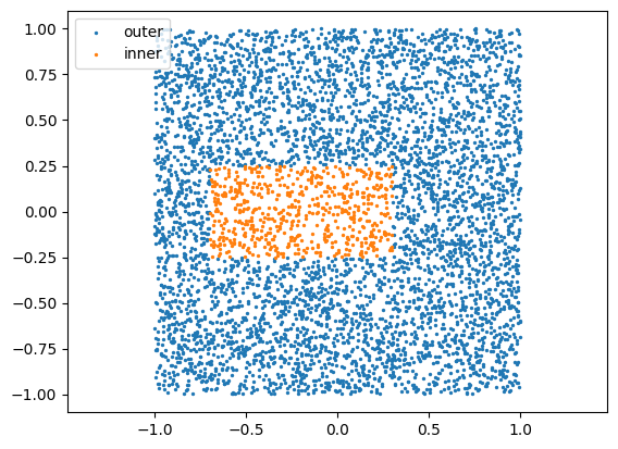
One can also specify the number of points per label:

key, dict_of_samples = sampler.sample(key, {"outer": 5000, "inner": 600})
for label in dict_of_samples:
    print("label: %s, %d points" % (label, dict_of_samples[label][0].shape[0]))

plot_dict_of_samples_2d(dict_of_samples)
plt.show()

label: outer, 5000 points
label: inner, 600 points

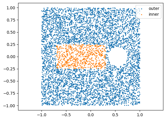
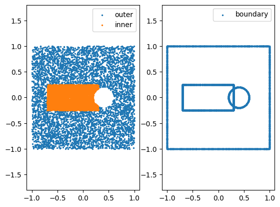
Holes

One can add holes to main domains:

from scimba_jax.domains.meshless_domains.domains_2d import Disk2D

center_h = (0.55, 0.0)
radius_h = 0.2
hole = Disk2D(center_h, radius_h, is_main_domain=False, label_str="hole")

print(hole)
print("\n")

big_square.add_hole(hole)

print(big_square)
print("\n")

sampler = DomainSampler(big_square)
key, dict_of_samples = sampler.sample(key, {"outer": 5000, "inner": 600})

plot_dict_of_samples_2d(dict_of_samples)
plt.show()

VolumetricDomain with label "hole" of type Disk2D sub-domain


VolumetricDomain with label "outer" of type Square2D main domain,
   - with subdomains: ["inner", ],
   - with holes: ["hole", ]

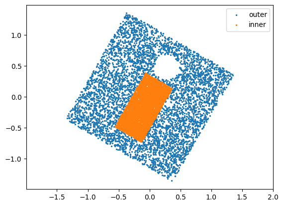
Mapped Geometric Domains

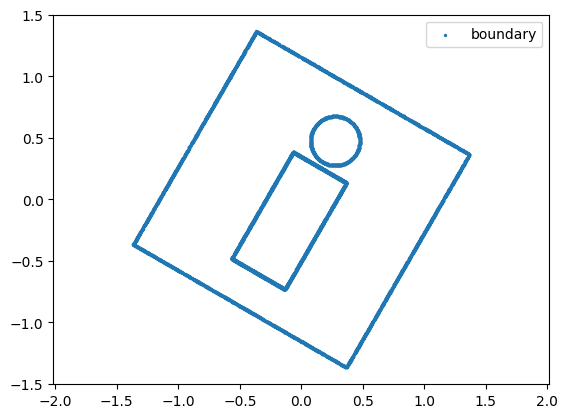
VolumetricDomains can be mapped, in which case the mapping is applied to its subdomains and to its holes. Here we apply a rotation of center \((0, 0)\) to our domain:

from scimba_jax.domains.domain_mapping import DomainMapping as Mapping

big_square.set_mapping(
    Mapping.rot_2d(
        angle=jnp.pi / 3.0,
        center=jnp.array([0.0, 0.0]),
    ),
    [(-2., 2.), (-2., 2.)],
)

sampler = DomainSampler(big_square)

key, dict_of_samples = sampler.sample(key, 10000)
plot_dict_of_samples_2d(dict_of_samples)
plt.show()

Boundaries of VolumetricDomain Objects

By default, in ScimBa, the boundaries of an object is the union of the geometric elements forming its borders. For example, for a Square2D object:

for bc in big_square.full_bc_domain():
    print(bc)

SurfacicDomain with label "bc south" of type Segment2D
SurfacicDomain with label "bc east" of type Segment2D
SurfacicDomain with label "bc north" of type Segment2D
SurfacicDomain with label "bc west" of type Segment2D

the boundaries is the union of the four \(2\)-dimensional segments.

Boundary elements of geometric objects in \(\mathbb{R}^d\) are parameterized subsets of \(\mathbb{R}^d\) with dimension \(d'<d\) and represented by instances of class SurfacicDomain.

For main domains, the boundary is, by default the union of the geometric elements forming its borders and the borders of its subdomains and holes:

bc, bc_subdomains, bc_holes = big_square.get_all_bc_domains()
boundaries = bc + bc_subdomains + bc_holes
for bc in boundaries:
    print(bc)

SurfacicDomain with label "bc south" of type Segment2D
SurfacicDomain with label "bc east" of type Segment2D
SurfacicDomain with label "bc north" of type Segment2D
SurfacicDomain with label "bc west" of type Segment2D
SurfacicDomain with label "bc hole circle" of type Circle2D
SurfacicDomain with label "bc inner south" of type Segment2D
SurfacicDomain with label "bc inner east" of type Segment2D
SurfacicDomain with label "bc inner north" of type Segment2D
SurfacicDomain with label "bc inner west" of type Segment2D

The default boundary is automatically constructed by the sampler, which has a method bc_sample to draw random points from the boundary:

key, dict_of_samples = sampler.bc_sample(key, 10000)

for label in dict_of_samples:
    print("label: %s, %d points" % (label, dict_of_samples[label][0].shape[0]))
print("\n")

plot_dict_of_samples_2d(dict_of_samples)
plt.show()

label: boundary, 10000 points

The method bc_samples returns points on the boundary and the normals of the boundaries at those points:

def plot_points_normals_2d(
    dict_of_samples: dict[str, tuple[jnp.ndarray, ...]],
    step:int = 10,
    scale=20., scale_units="width",
    fig=None, index=111,
):
    if fig is None:
        fig = plt.figure()
    axe=fig.add_subplot(index)
    for label in dict_of_samples:
        x, y = dict_of_samples[label][0][::step,0], dict_of_samples[label][0][::step,1]
        axe.scatter(x, y, s=2, label=label)
        u, v = dict_of_samples[label][1][::step,0], dict_of_samples[label][1][::step,1]
        axe.quiver(x, y, u, v, label=label + " normals", scale=scale, scale_units=scale_units)
    axe.legend()
    axe.axis('equal')
    return fig

plot_points_normals_2d(dict_of_samples)
plt.show()

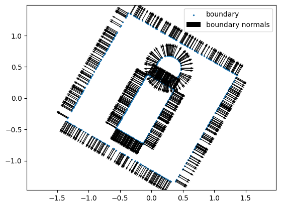
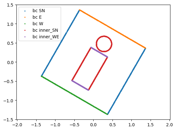
By default, all the boundary elements are grouped together. However, if you need to apply different constraints to different areas of boundaries, you can define boundary groups as a dictionary:

big_square.set_boundaries_dict(
    {
        "bc SN": ["bc south", "bc north"],
        "bc E": ["bc east"],
        "bc W": ["bc west"],
        "bc inner_SN": ["bc inner south", "bc inner north", "bc hole circle"],
        "bc inner_WE": ["bc inner west", "bc inner east"],
    }
)

sampler = DomainSampler(big_square)
key, dict_of_samples = sampler.bc_sample(key, 10000)

for label in dict_of_samples:
    print("label: %s, %d points" % (label, dict_of_samples[label][0].shape[0]))
print("\n")

plot_dict_of_samples_2d(dict_of_samples)
plt.show()

label: bc SN, 2223 points
label: bc E, 1111 points
label: bc W, 1111 points
label: bc inner_SN, 3333 points
label: bc inner_WE, 2222 points

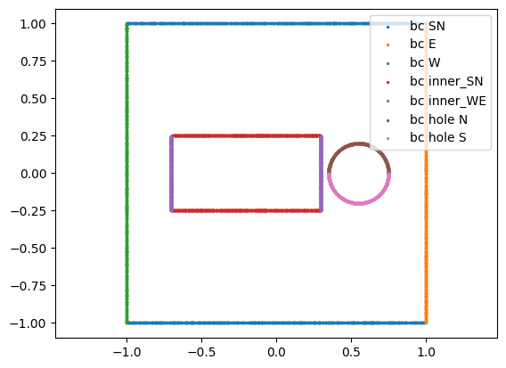
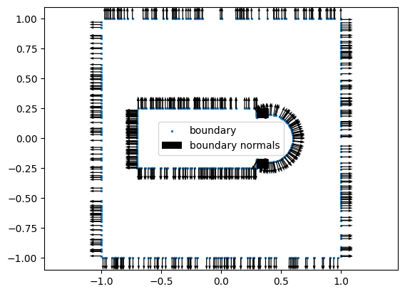
Custom Boundary Definition

Suppose you want to apply different constraints based the position on the boundary of the circular hole:

from scimba_jax.domains.meshless_domains.domains_2d import ArcCircle2D, Disk2D

center_h = (0.55, 0.0)
radius_h = 0.2
hole = Disk2D(center_h, radius_h, is_main_domain=False, label_str="hole")
disk_up = ArcCircle2D(center_h, radius_h, (0.0, jnp.pi), label_str="bc hole north")
disk_do = ArcCircle2D(center_h, radius_h, (jnp.pi, 2 * jnp.pi), label_str="bc hole south")
hole.add_bc_domain(disk_up)
hole.add_bc_domain(disk_do)

print(hole)

VolumetricDomain with label "hole" of type Disk2D sub-domain,
   - with boundaries: [
      -- "boundary": ["bc hole north", "bc hole south", ]
     ]

big_square = Square2D(bounds_o, is_main_domain=True, label_str="outer")
small_square = Square2D(bounds_i, is_main_domain=False, label_str="inner")
big_square.add_subdomain(small_square)
big_square.add_hole(hole)

big_square.set_boundaries_dict(
    {
        "bc SN": ["bc south", "bc north"],
        "bc E": ["bc east"],
        "bc W": ["bc west"],
        "bc inner_SN": ["bc inner south", "bc inner north"],
        "bc inner_WE": ["bc inner west", "bc inner east"],
        "bc hole N": ["bc hole north"],
        "bc hole S": ["bc hole south"],
    }
)

sampler = DomainSampler(big_square)
key, dict_of_samples = sampler.bc_sample(key, 10000)

for label in dict_of_samples:
    print("label: %s, %d points" % (label, dict_of_samples[label][0].shape[0]))
print("\n")

plot_dict_of_samples_2d(dict_of_samples)
plt.show()

label: bc SN, 2000 points
label: bc E, 1000 points
label: bc W, 1000 points
label: bc inner_SN, 2000 points
label: bc inner_WE, 2000 points
label: bc hole N, 1000 points
label: bc hole S, 1000 points

Holes and Boundaries

Holes are applied to interiors of domains and subdomains but not to their boundaries:

bounds_o = [(-1.0, 1.0), (-1.0, 1.0)]
bounds_i = [(-0.7, 0.3), (-0.25, 0.25)]
big_square = Square2D(bounds_o, is_main_domain=True, label_str="outer")
small_square = Square2D(bounds_i, is_main_domain=False, label_str="inner")
big_square.add_subdomain(small_square)

center_h = (0.4, 0.0)
radius_h = 0.2
hole = Disk2D(center_h, radius_h, is_main_domain=False, label_str="hole")

big_square.add_hole(hole)

sampler = DomainSampler(big_square)
key, dict_of_samples = sampler.sample(key, 10000)

fig = plot_dict_of_samples_2d(dict_of_samples, index=121)

key, dict_of_samples = sampler.bc_sample(key, 10000)
plot_dict_of_samples_2d(dict_of_samples, fig=fig, index=122)
plt.show()

In such a case, you must define a custom boundary:

import math
from scimba_jax.domains.meshless_domains.domains_2d import Segment2D


big_square = Square2D(bounds_o, is_main_domain=True, label_str="outer")
small_square = Square2D(bounds_i, is_main_domain=False, label_str="inner")

hole = Disk2D(center_h, radius_h, is_main_domain=False, label_str="hole")
arc = ArcCircle2D(center_h, radius_h, (-2*jnp.pi/3, 2*jnp.pi/3.), label_str="bc hole")
hole.add_bc_domain(arc)

# define boundary elements of inner square \setminus the hole
y_inter = radius_h*math.sqrt(3.)/2.
small_square.list_bc_domains = [
    Segment2D((-0.7, -0.25), (0.3, -0.25), label_str = "bc inner south"),
    Segment2D((0.3, 0.25), (-0.7, 0.25), label_str = "bc inner north"),
    Segment2D((-0.7, 0.25), (-0.7, -0.25), label_str = "bc inner west"),
    Segment2D((0.3, -0.25), (0.3, -y_inter), label_str = "bc inner s east"),
    Segment2D((0.3, y_inter), (0.3, 0.25), label_str = "bc inner n east"),
] #notice the orders in which the boundaries of the segments are given
big_square.add_subdomain(small_square)

big_square.add_hole(hole)

sampler = DomainSampler(big_square)

key, dict_of_samples = sampler.bc_sample(key, 10000)
plot_points_normals_2d(dict_of_samples, scale=30)
plt.show()

Temporal/parametric/kinetic Domains and Samplers

It is easy to handle time dependent, parametric and kinetic problems in ScimBa:

• time domains are represented by real intervals,

• parameters domains are represented by carthesian products of real intervals.

from scimba_jax.nonlinear_approximation.integration.monte_carlo_time import (
    UniformTimeSampler,
)
from scimba_jax.nonlinear_approximation.integration.monte_carlo_parameters import (
    UniformParametricSampler,
)

domain_t = (0.0, 1.0)

t_sampler = UniformTimeSampler(domain_t)

domain_mu = [(0.0, 1.0), (2., 3.)]

mu_sampler = UniformParametricSampler(domain_mu)

For kinetic problems, velocity values can be drawn from a 2D circle:

from scimba_jax.nonlinear_approximation.integration.monte_carlo_parameters import (
    UniformVelocitySampler,
)
from scimba_jax.domains.meshless_domains.domains_2d import Circle2D

domain_v = Circle2D((0.0, 0.0), 1.)

v_sampler = UniformVelocitySampler(domain_v)

key, samples = v_sampler.sample(key, 5)

print(samples)

[[-0.36141196 -0.93240624]
 [ 0.96575759 -0.25944611]
 [-0.97882589 -0.20469457]
 [-0.92292651 -0.38497618]
 [ 0.9940614   0.10882066]]

Or from a 1D segment:

from scimba_jax.nonlinear_approximation.integration.monte_carlo_parameters import (
    UniformVelocitySamplerOnCuboid,
)

domain_v = Segment1D((0.0, 1.0))
v_sampler = UniformVelocitySamplerOnCuboid(domain_v)
key, samples = v_sampler.sample(key, 5)

print(samples)

[[0.80605648]
 [0.85350797]
 [0.50245583]
 [0.99936948]
 [0.69520571]]

Or from a 2D rectangle:

domain_v = Square2D([(0.0, 1.0)]*2)
v_sampler = UniformVelocitySamplerOnCuboid(domain_v)
key, samples = v_sampler.sample(key, 5)

print(samples)

[[0.73704278 0.4451332 ]
 [0.29600371 0.25958073]
 [0.84339186 0.56026991]
 [0.54181534 0.31815042]
 [0.40690713 0.07605483]]

Tensorized Samplers for Global Domains

Below, we demonstrate how to create a sampler for a stationary, kinetic and parametric problem by gathering samplers for geometric, kinetic and parametric domains in a TensorizedSampler:

from scimba_jax.nonlinear_approximation.integration.monte_carlo import (
    TensorizedSampler,
)

domain_mu = [(0., 1.), (2., 3.), (4., 5.)]
domain_v = Segment1D((0.0, 1.0))

sampler = TensorizedSampler(
    [
        DomainSampler(big_square),
        UniformVelocitySamplerOnCuboid(domain_v),
        UniformParametricSampler(domain_mu),
    ],
    model_type="x_v_mu",
    bc=True,
)

The optional argument model_type specifies the names of the sampled variables.

The optional argument bc, which defaults to True, indicates whether the sampler must draw random points on the boundary of the geometric domain.

The sample method of the sampler takes in input, in addition to the random state, the number of points to sample on the interior and on the boundaries:

key, dict_of_samples = sampler.sample(key, n=10, n_bc=10)

print(dict_of_samples.keys())
print("\n")

print(dict_of_samples["inner"])

dict_keys(['outer', 'inner', 'boundary'])


(Array([[ 0.20614475, -0.14289075],
       [-0.04140162, -0.00659051],
       [-0.23384062,  0.07448716],
       [-0.18438006, -0.07498472],
       [-0.23894359,  0.10383828]], dtype=float64), Array([[0.96672101],
       [0.03622169],
       [0.81613051],
       [0.17371903],
       [0.05327374]], dtype=float64), Array([[0.73359158, 2.15125924, 4.33834824],
       [0.03899169, 2.54975422, 4.24799535],
       [0.66679419, 2.1394429 , 4.5196841 ],
       [0.62667889, 2.12518822, 4.30985557],
       [0.22410455, 2.72306047, 4.25054416]], dtype=float64))

For a temporal parametric problem:

domain_t = (0.0, 1.0)
sampler = TensorizedSampler(
    [
        UniformTimeSampler(domain_t),
        DomainSampler(big_square),
        UniformParametricSampler(domain_mu),
    ],
    model_type="t_x_mu",
    bc=True,
    ic=True
)

The ic optional argument, which is True by default, indicates weither the sampler must draw random points for the initial time.

key, dict_of_samples = sampler.sample(key, n=10, n_bc=10, n_ic = 3)

print(dict_of_samples.keys())
print("\n")

print(dict_of_samples["ic inner"])

dict_keys(['outer', 'inner', 'boundary', 'ic outer', 'ic inner'])


(Array([[-0.27248921,  0.1549125 ]], dtype=float64), Array([[0.4098706 , 2.82845126, 4.81299965]], dtype=float64))

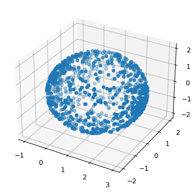
Creating Custom Domains `scimba_jax

In this section, we will create two new types of 3D domains:

• 3D spheres, which are SurfacicDomains,

• and 3D balls, which are VolumetricDomains and have 3D spheres as boundary.

Creating Custom Surfacic Domains

SurfacicDomain subclasses implement parameterized surfaces, and are characterized by:

• the parameterization, which is a function encapsulated in class called DomainMapping,

• the parameter’s domain which is a VolumetricDomain.

Let us define a classical parameterization for a 3D ball:

def sphere_parameterization(x: jnp.ndarray, center: jnp.ndarray, radius: float):
    return (
        center + jnp.concatenate([
            jnp.cos(x[0:1]),
            jnp.sin(x[0:1]) * jnp.cos(x[1:2]),
            jnp.sin(x[0:1]) * jnp.sin(x[1:2]),
        ],axis=-1) * radius
    )

Important remark: the parameterization must be defined for a single vector of parameters, not a batch, as it will be vmapped.

When \(x\in [0, \pi]\times[0,2\pi]\) this parameterizes a sphere:

center = (1., 0., 0.)
radius = 2.
N_POINTS = 1000

key, keyt, keyp = jax.random.split(key, 3)
theta = jax.random.uniform(keyt, shape=(N_POINTS, 1), minval=0., maxval=jnp.pi)
phi = jax.random.uniform(keyp, shape=(N_POINTS, 1), minval=0., maxval=2*jnp.pi)
angles = jnp.concatenate([theta, phi], axis=-1)
sphere = jax.vmap(sphere_parameterization, in_axes=(0, None, None))(
    angles,
    jnp.array(center),
    radius
)
ax = plt.figure().add_subplot(projection="3d")
x, y, z = sphere[:,0], sphere[:,1], sphere[:,2]
ax.scatter(x, y, z, label=label)
plt.show()

Next we encapsulate the parameterization in a DomainMapping instance:

from scimba_jax.domains.domain_mapping import DomainMapping

def make_sphere_mapping(center: jnp.ndarray, radius: float):
    return DomainMapping(
        from_dim = 2,
        to_dim = 3,
        map = lambda x: sphere_parameterization(x, center, radius),
    )

sphere_mapping = make_sphere_mapping(jnp.array(center), radius)

This allows us, among others, to evaluate derivatives of the mapping (and this is useful for computing normals to the surface):

def jac_sphere_parameterization(x: jnp.ndarray, center: jnp.ndarray, radius: float):
    dt1 = jnp.concatenate([
            -jnp.sin(x[0:1]),
            jnp.cos(x[0:1]) * jnp.cos(x[1:2]),
            jnp.cos(x[0:1]) * jnp.sin(x[1:2]),
    ],axis=-1)
    dt2 = jnp.concatenate([
            jnp.zeros_like(x[0:1]),
            -jnp.sin(x[0:1]) * jnp.sin(x[1:2]),
            jnp.sin(x[0:1]) * jnp.cos(x[1:2]),
    ],axis=-1)
    return radius * jnp.stack([dt1, dt2], axis=-1)

jac_1 = sphere_mapping.evaluate_jacobian(angles)
jac_2 = jax.vmap(jac_sphere_parameterization, in_axes=(0, None, None))(
    angles,
    jnp.array(center),
    radius
)
assert jnp.allclose(jac_1, jac_2)

Once the parameterization is ready, one can define the Sphere3D class which inherits from SurfacicDomain:

from scimba_jax.domains.meshless_domains.base import SurfacicDomain

class Sphere3D(SurfacicDomain):
    def __init__(
        self,
        center: jnp.ndarray | tuple[float, float],
        radius: float,
        label_str: str = "boundary",
        label_idx: int = 0,
    ):
        if not isinstance(center, jnp.ndarray):
            center = jnp.array(center, dtype=scimba_jax.get_default_dtype())
        if not center.shape == (3,):
            raise ValueError("center must be a tensor of shape (3,)")

        super(Sphere3D, self).__init__(
            domain_type="Sphere3D",
            parametric_domain=Square2D([(0.0, jnp.pi), (0.0, 2 * jnp.pi)]),
            surface=make_sphere_mapping(center, radius),
            label_str=label_str,
            label_idx=label_idx,
        )
        self.center = center
        self.radius = radius

sphere = Sphere3D(center, radius)
print(sphere)

SurfacicDomain with label "boundary" of type Sphere3D

Notice the parametric domain which is here a Square2Dobject.

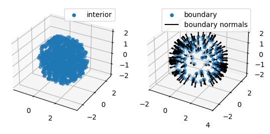
Creating Custom Volumetric Domains

To implement a subclass of VolumetricDomain representing a type of sets, one must provide a function to test membership in the form of a Signed Distance Function (SDF). See for instance:

[Sukumar2022] N. Sukumar, Ankit Srivastava. Exact imposition of boundary conditions with distance functions in physics-informed deep neural networks. Computer Methods in Applied Mechanics and Engineering, Volume 389, 2022, 114333.

Such SDFs must be subclasses of SignedDistancewhich is itself a DomainMapping. We reproduce the definition of SignedDistance below.

from abc import abstractmethod

class SignedDistance(DomainMapping):
    def __init__(self, dim: int, threshold: float = 0.0):
        super(SignedDistance, self).__init__(
            dim, 1, self._sdf_pointwise, None, None, None
        )
        self.dim = dim
        self.threshold = threshold
        self.sdf = self.evaluate
        self.sdf_pointwise = self.evaluate_pointwise

    @abstractmethod
    def _sdf_pointwise(self, x: jnp.ndarray) -> jnp.ndarray:
        """The sdf at a point."""

The SDF for an ND ball is straightforward:

class BallNDSignedDistance(SignedDistance):
    def __init__(self, center: jnp.ndarray, radius: float):
        if not (center.ndim == 1):
            raise ValueError("first argument must be a jnp array of shape (d,)")
        dim = center.shape[0]
        super().__init__(dim, threshold=0.0)
        self.center = center
        self.radius = radius

    def _sdf_pointwise(self, x):
        return (jnp.linalg.norm(x - self.center, axis=0) - self.radius)[None]

One can now use this SDF to define the class representing 3D balls:

from scimba_jax.domains.meshless_domains.base import VolumetricDomain

class Ball3D(VolumetricDomain):
    def __init__(
        self,
        center: jnp.ndarray | tuple[float, float, float],
        radius: float,
        is_main_domain=False,
        label_str: str = "interior",
        label_idx: int = 0,
    ):
        if not isinstance(center, jnp.ndarray):
            center = jnp.array(center, dtype=scimba_jax.get_default_dtype())
        if not (center.shape == (3,)):
            raise ValueError("center must be a tensor of shape (3,)")

        super(Ball3D, self).__init__(
            domain_type="Ball3D",
            dim=3,
            sdf=BallNDSignedDistance(center, radius),
            bounds=[
                (center[i].item() - radius, center[i].item() + radius)
                for i in range(3)
            ],
            is_main_domain=is_main_domain,
            label_str=label_str,
            label_idx=label_idx,
        )
        self.center = center
        self.radius = radius

    def full_bc_domain(self) -> list[SurfacicDomain]:
        label_bc = "bc"
        if not self.is_main_domain:
            label_bc += " " + self.get_label()
        res = Sphere3D(self.center, self.radius, label_str=label_bc + " sphere")
        if self.is_mapped:
            res._set_mapping(self.mapping)
        return [res]

In full_bc_domain, the boundary is constructed as an instance of Sphere3D.

Let us instantiate and plot our object:

ball = Ball3D(center, radius, is_main_domain=True)

print(ball)

VolumetricDomain with label "interior" of type Ball3D main domain

def plot_dict_of_samples_3d(
    dict_of_samples: dict[str, tuple[jnp.ndarray, ...]],
    fig=None, index=111
):
    if fig is None:
        fig = plt.figure()
    axe=fig.add_subplot(index, projection="3d")
    for label in dict_of_samples:
        x = dict_of_samples[label][0][:,0]
        y = dict_of_samples[label][0][:,1]
        z = dict_of_samples[label][0][:,2]
        axe.scatter(x, y, z, label=label)
        axe.legend()
        axe.axis("equal")
    return fig

def plot_points_normals_3d(
    dict_of_samples: dict[str, tuple[jnp.ndarray, ...]],
    step:int = 10, length:float=0.5, fig=None, index=111
):
    if fig is None:
        fig = plt.figure()
    axe=fig.add_subplot(index, projection="3d")
    for label in dict_of_samples:
        x = dict_of_samples[label][0][::step,0]
        y = dict_of_samples[label][0][::step,1]
        z = dict_of_samples[label][0][::step,2]
        axe.scatter(x, y, z, label=label)
        u = dict_of_samples[label][1][::step,0]
        v = dict_of_samples[label][1][::step,1]
        w = dict_of_samples[label][1][::step,2]
        axe.quiver(x, y, z, u, v, w, label=label + " normals", color='black', length=length)
        axe.legend()
        axe.axis("equal")
    return fig

sampler = DomainSampler(ball)

key, dict_of_samples = sampler.sample(key, N_POINTS)

fig = plot_dict_of_samples_3d(dict_of_samples, index=121)

key, dict_of_samples = sampler.bc_sample(key, N_POINTS)

fig = plot_points_normals_3d(dict_of_samples, step=5, fig=fig,index=122)
plt.show()

Generic domains

Scimba_jax provides ready-to-use domains in arbitrary dimensions:

• Hypercubes and their faces called hypersquares,

• \(N\) dimensional balls and \(N-1\)-spheres.

Hypercubes

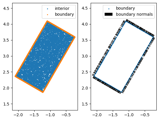
In dimension 2, hypercubes are rectangles:

from scimba_jax.domains.meshless_domains.domains_nd import HypercubeND

bounds = [(1.0, 3.0), (2.0, 3.0)]
square = HypercubeND(bounds, is_main_domain=True)

square.set_mapping(
    Mapping.rot_2d(
        angle=jnp.pi / 3.0,
        center=jnp.array([0.0, 0.0]),
    ),
    [(-2., 2.), (-2., 2.)],
)

sampler = DomainSampler(square)

key, dict_of_samples = sampler.sample(key, 10000)
key, dict_of_samples_bc = sampler.bc_sample(key, 10000)
dict_of_samples = dict_of_samples | dict_of_samples_bc

fig = plot_dict_of_samples_2d(dict_of_samples, index=121)
plot_points_normals_2d(dict_of_samples_bc, scale=30, fig=fig, index=122)
plt.show()

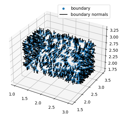
In dimension 3:

bounds = [(1.0, 3.0), (2.0, 3.0), (2.0, 3.0)]
cube = HypercubeND(bounds, is_main_domain=True)

sampler = DomainSampler(cube)

key, dict_of_samples_bc = sampler.bc_sample(key, 1000)

plot_points_normals_3d(dict_of_samples_bc, step=1, length=0.1)
plt.show()

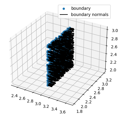
The boundaries of hypercubes in \(N\) dimensions are \(2N\) hypersquares that are hypercubes in \(N-1\) dimensions embedded in \(\mathbb{R}^N\).

from scimba_jax.domains.meshless_domains.domains_nd import HypersquareND

bounds = [(1.0, 3.0), (2.0, 3.0), (2.0, 3.0)]
cube = HypercubeND(bounds, is_main_domain=True)

cube.list_bc_domains = [
    HypersquareND(origin=[3., 2., 2.], basis=jnp.eye(3)[1:],label_str = "bc 1"),
] #notice the orders in which the boundaries of the segments are given

sampler = DomainSampler(cube)

key, dict_of_samples_bc = sampler.bc_sample(key, 1000)

plot_points_normals_3d(dict_of_samples_bc, step=1, length=0.1)
plt.show()

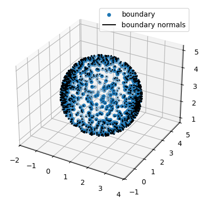
\(N\) dimensional balls

from scimba_jax.domains.meshless_domains.domains_nd import BallND

ball = BallND(center=[1, 2, 3], radius=2., is_main_domain=True)

sampler = DomainSampler(ball)

key, dict_of_samples_bc = sampler.bc_sample(key, 1000)

plot_points_normals_3d(dict_of_samples_bc, step=1, length=0.1)
plt.show()