Scimba basics I: approximation of the solution of pre-defined physical models

In this first tutorial, we will walk you through the basics of scimba_jax for defining and training Physics-Informed Neural Networks (PINNs) for two toy examples, a stationary one and a time dependent one.

Scimba and jax setting

Scimba_jax is based on jax for tensor arithmetic, auto-differentiation, neural networks definition and evaluation, etc.

At initialization, Scimba sets jax default floating point format to double. We discourage using float32 as default type (Natural Gradient descent, which is the default optimization used in Scimba_jax, requires precision).

The default device for tensors computation is jax default device; here we are using a Cuda device:

import jax
import jax.numpy as jnp
import scimba_jax

See version (scimba_jax is experimental so far), floating arithmetic precision and current device with:

scimba_jax.set_verbosity(True)
scimba_jax.set_verbosity(False)

/////////////// Scimba jax 0.0.1 ////////////////
Scimba_jax uses device: [CudaDevice(id=0)]
Scimba_jax uses dtype: <class 'jax.numpy.float64'>

The device can be changed with the jax API:

print("GPUs :", jax.devices("gpu"))
print("CPU :", jax.devices("cpu"))
jax.config.update("jax_default_device", jax.devices("cpu")[0])
print("Scimba_jax uses device:", jax.devices())
a = jnp.ones(5)
print("default device: ", a.device)

GPUs : [CudaDevice(id=0)]
CPU : [CpuDevice(id=0)]
Scimba_jax uses device: [CudaDevice(id=0)]
default device:  TFRT_CPU_0

jax.config.update("jax_default_device", jax.devices("gpu")[0])
a = jnp.ones(5)
print("default device: ", a.device)

default device:  cuda:0

Approximation of the solution of a parametric 2D Laplacian

We consider the equation:

\[- \mu \Delta u = 2(\mu\pi)^2 \sin(\pi x) \sin(\pi y)\]

on \((x,y) \in \Omega := [-1, 1]\times[-1, 1]\) with parameter \(\mu\in \mathbb{M}=[1,2]\) subject to the Dirichlet condition:

\[u = 0\]

on \(\partial\Omega\).

Geometric domain \(\Omega \subset \mathbb{R}^2\)

In Scimba, in a \(d\)-dimensional ambiant space,

• \(d\)-dimensional geometric domains are objects of class VolumetricDomain, and

• \(d-1\)-dimensional geometric domains are objects of class SurfacicDomain.

Most common types of domains (carthesian products of intervals, disks, …) are implemented in scimba_torch.domains.meshless_domain.domains_Nd (with N\(=1\) or \(2\)).

Here, we define \(\Omega := [-1, 1]\times[-1, 1]\) with:

from scimba_jax.domains.meshless_domains.domains_2d import Square2D

domain_x = Square2D([(-1.0, 1.0), (-1.0, 1.0)], is_main_domain=True)

The keyword argument is_main_domain indicates whether the created object is a main domain or is a subdomain of a main domain; Scimba allows to create complex geometries by combining holes and subdomains.

Sampler on \(\Omega\times \mathbb{M}\)

The next step is to define samplers for geometric and parameter’s domains. The module scimba_jax.nonlinear_approximation.integration provides uniform samplers for physical and parameter’s domains.

from scimba_jax.nonlinear_approximation.integration.monte_carlo import (
    DomainSampler,
    TensorizedSampler,
)
from scimba_jax.nonlinear_approximation.integration.monte_carlo_parameters import (
    UniformParametricSampler,
)

domain_mu = [(1., 2.)]
sampler = TensorizedSampler(
    [DomainSampler(domain_x), UniformParametricSampler(domain_mu)], bc=True
)

A tensorized sampler gathers samplers for the domains of the variables of the problem. Notice the optional argument bc=True which tells the sampler to sample boundaries of the geometric domain.

Right-hand side and exact solution

Next we define the right-hand side of the residual and, since we know it, the analytical expression of the solution. We will use it to compare with the computed approximate solution.

def f_rhs(xy: jnp.ndarray, mu: jnp.ndarray) -> jnp.ndarray:
    x, y = xy[..., 0:1], xy[..., 1:2]
    return 2 * (mu[...,0:1] * jnp.pi)**2 * jnp.sin(jnp.pi * x) * jnp.sin(jnp.pi * y)

def analytic_solution(xy: jnp.ndarray, mu: jnp.ndarray) -> jnp.ndarray:
    x, y = xy[..., 0:1], xy[..., 1:2]
    return mu * jnp.sin(jnp.pi * x) * jnp.sin(jnp.pi * y)

Physical model

Several PDEs are implemented in Scimba and ready-to-use; here we use the 2D Laplacian in strong form with Dirichlet boundary condition:

from scimba_jax.physical_models.elliptic_pde.laplacians import ParametricLaplacianDirichletND

model = ParametricLaplacianDirichletND(domain_x, f_rhs, bc="weak")

One can also taylor its own model as described in next tutorials.

Here the right-hand side of the Dirichlet boundary condition is the zero function; when it is not the case, one must define it, then pass it throught the named argument f_bc_rhs when constructing the model.

In scimba_torch, the right-hand side for boundary condition residual takes also the normals in input.

def f_bc_rhs(xy: jnp.ndarray, n: jnp.ndarray, mu: jnp.ndarray) -> jnp.ndarray:
    x = xy[..., 0:1]
    return jnp.zeros_like(x)

model = ParametricLaplacianDirichletND(domain_x, f_rhs, bc="weak", f_bc_rhs=f_bc_rhs)

Approximation space

In Scimba, the solution of a PDE is approximated by an element \(u_{\theta}\) of a set of parameterized functions called approximation space.

Here we wish to approximate the solution with a Multi-Layer Perceptron with 3 scalar input (\(x,y\) and \(\mu\)), 1 output (\(u(x,y,\mu)\)) and three intermediate layers of \(16\) neurons each:

from scimba_jax.nonlinear_approximation.networks.mlp import MLP
from scimba_jax.nonlinear_approximation.approximation_spaces.approximation_spaces import (
    ApproximationSpace,
)

key = jax.random.PRNGKey(0) #initialize the random generator

nn = MLP(in_size=3, out_size=1, hidden_sizes=[16, 16], key=key)
space = ApproximationSpace(
    {"x": 2, "mu": 1},       # x has dim 2, mu has dim 1
    [(nn, "scalar", None)],  # nn models a scalar function u
    model_type="x_mu",       # u depends of x and mu
)

Scimba PINN

We finally create a PINN as an instance of the class Projector:

from scimba_jax.nonlinear_approximation.numerical_solvers.projectors import Projector

pinn = Projector(model, space, sampler, matrix_regularization=1e-5)

The default optimizer used in scimba_jax PINNs is Natural Gradient descent (see below); the optional argument matrix_regularization is an important parameter used in this optimizer; by default, it takes value 1e-6.

The pinn is not trained yet; let us sample some collocation points and evaluate the losses functions associated to the interior residual and the boundary residual of the model:

N_COLLOC = 1000 # the number of collocation points for the interior residual
N_BC_COLLOC = 1000 # the number of collocation points for the boundary residual
key, sample_dict = sampler.sample(key, N_COLLOC, N_BC_COLLOC)

losses = pinn.evaluate_losses(space, sample_dict)

print("interior loss before training: ", losses["interior"])
print("boundary loss before training: ", losses["boundary"])
print("total    loss before training: ", losses["total"])

interior loss before training:  [591.51702936]
boundary loss before training:  [0.0798538]
total    loss before training:  592.3155673139493

The total loss is a weighted sum of the losses. By default the weights are:

• \(1\) for the interior residual

• \(10\) for the boundary residual (and the initial residual for time dependent problems)

We will show later how to adjust those weights.

How to train the PINN:

By default, scimba_jax PINNs are trained with Energy Natural Gradient preconditioned gradient descent:

import timeit

N_EPOCHS = 50

start = timeit.default_timer()
key, pinn = pinn.project(key, space, N_EPOCHS, N_COLLOC, N_BC_COLLOC)
end = timeit.default_timer()

print("time for %d epochs: " % N_EPOCHS, end - start)

print("interior loss after training: ", pinn.best_loss["interior"])
print("boundary loss after training: ", pinn.best_loss["boundary"])
print("total    loss after training: ", pinn.best_loss["total"])

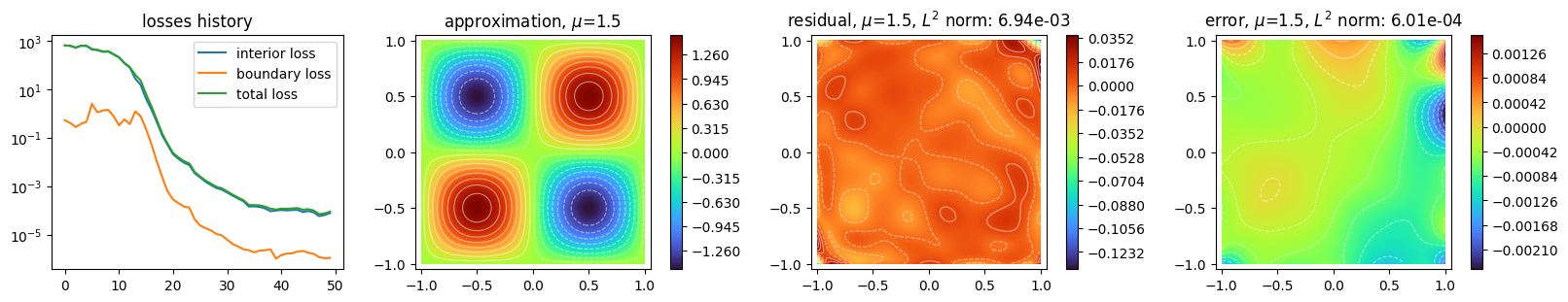
Training: 100%|||||||||||||||||||| 50/50[00:20<00:00] , loss: 6.4e+02 -> 7.0e-05
time for 50 epochs:  20.4095377670601
interior loss after training:  [5.81954077e-05]
boundary loss after training:  [1.16094794e-06]
total    loss after training:  6.980488710483936e-05

the trainnig loop returns:

• a state for the random generator (key),

• a modified projector; the trained approximation space is accessed through pinn.space.

Plot the training of a PINN:

For graphical output:

import matplotlib.pyplot as plt

from scimba_jax.plots.plots_nd import plot_abstract_approx_space

plot_abstract_approx_space(
    pinn.space,  # the approximation space
    domain_x,  # the spatial domain
    domain_mu,  # the parameter's domain
    loss=pinn.losses,  # for plot of the loss: the losses
    residual=pinn.model,  # for plot of the residual: the pde
    error=analytic_solution,  # for plot of the error with respect to a func: the func
    draw_contours=True,
    n_drawn_contours=20,
)
plt.show()

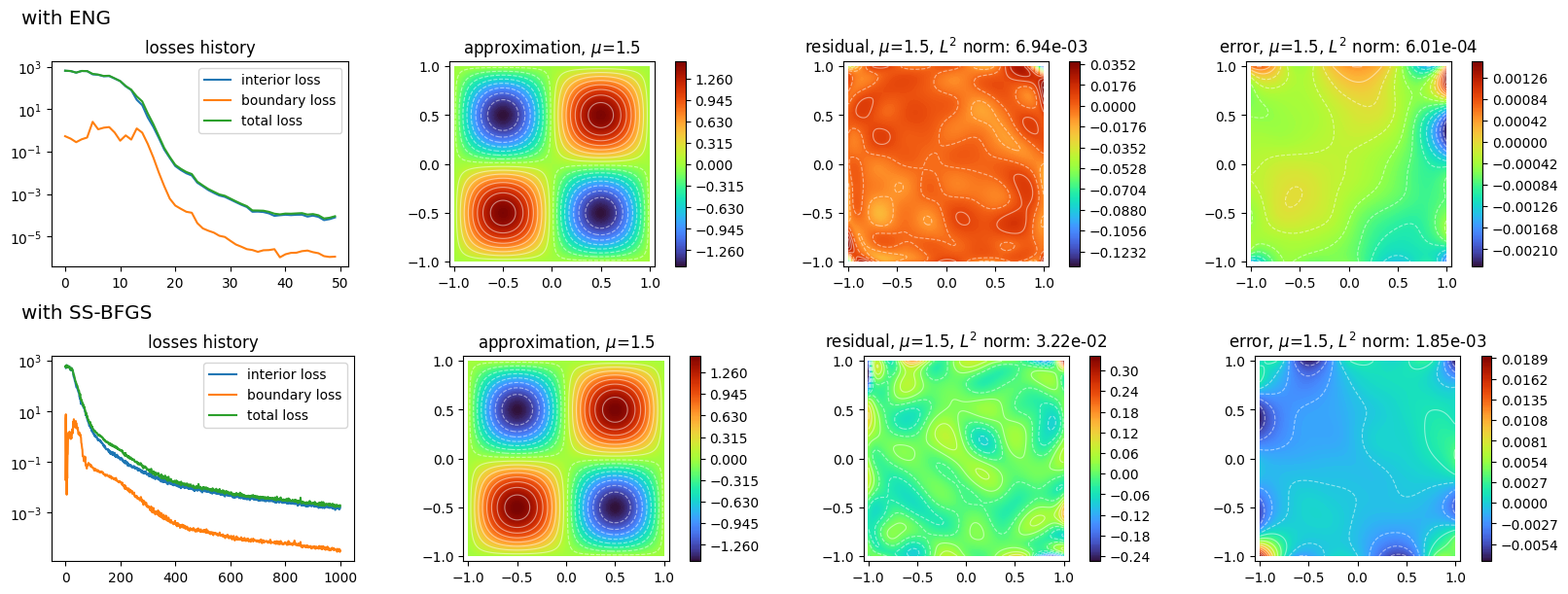
How to select an optimizer

Several optimizers are implemented in scimba_jax:

• Natural gradient descent: ENG and ANaGRAM

• Adam

• L-BFGS

• SS-BFGS and SS-Broyden as described here.

The optimizer to use has to be specified at the instantiation of the PINN:

key = jax.random.PRNGKey(0)

nn2 = MLP(in_size=3, out_size=1, hidden_sizes=[16, 16, 16], key=key)
space2 = ApproximationSpace(
    {"x": 2, "mu": 1},       # x has dim 2, mu has dim 1
    [(nn2, "scalar", None)],  # nn models a scalar function u
    model_type="x_mu",       # u depends of x and mu
)

pinn2 = Projector(model, space2, sampler, optimizer="SS-BFGS")

N_EPOCHS_SSBFGS = 1000

start = timeit.default_timer()
key, pinn2 = pinn2.project(key, space2, N_EPOCHS_SSBFGS, N_COLLOC)
end = timeit.default_timer()

print("time for %d epochs: " % N_EPOCHS_SSBFGS, end - start)

print("interior loss after training: ", pinn2.best_loss["interior"])
print("boundary loss after training: ", pinn2.best_loss["boundary"])
print("total    loss after training: ", pinn2.best_loss["total"])

Training: 100%|||||||||||||||| 1000/1000[00:59<00:00] , loss: 6.3e+02 -> 1.6e-03
time for 1000 epochs:  59.80503505188972
interior loss after training:  [0.00125617]
boundary loss after training:  [3.45972324e-05]
total    loss after training:  0.0016021428376873275

The valid optimizer names are: “ENG”, “ANaGRAM”, “Adam”, “L-BFGS”, “SS-BFGS” and “SS-Broyden”.

Plot several pinns on the same figure

from scimba_jax.plots.plots_nd import plot_abstract_approx_spaces

plot_abstract_approx_spaces(
    (pinn.space, pinn2.space),  # the approximation spaces
    domain_x,  # the spatial domain
    domain_mu,  # the parameter's domain
    loss=(pinn.losses, pinn2.losses),  # for plot of the loss: the losses
    residual=(pinn.model, pinn2.model),  # for plot of the residual: the pde
    error=analytic_solution,  # for plot of the error with respect to a func: the func
    draw_contours=True,
    n_drawn_contours=20,
    titles=("with ENG", "with SS-BFGS"),
)
plt.show()

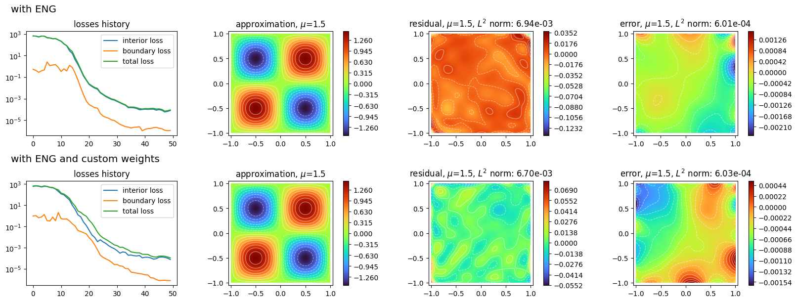
How to change the respective weigths of the equations of the residuals

Say one want to increase the weight of the boundary condition residual in the loss computation:

custom_weights = {"interior": [1.0], "boundary": [40.0]}

The label "interior" is given by default to:

• the interior of the main geometric domain

• the residual for the interior of the main geometric domain

• the loss assosiated to the residual for the interior of the main geometric domain whereas "boundary"is given by default to:

• the boundary of the main geometric domain

• the residual for the boundary of the main geometric domain

• the loss assosiated to the residual for the boundary of the main geometric domain.

Next create a new PINN using those weights:

key = jax.random.PRNGKey(0)

nn3 = MLP(in_size=3, out_size=1, hidden_sizes=[16, 16], key=key)
space3 = ApproximationSpace(
    {"x": 2, "mu": 1},       # x has dim 2, mu has dim 1
    [(nn3, "scalar", None)],  # nn models a scalar function u
    model_type="x_mu",       # u depends of x and mu
)

pinn3 = Projector(model, space3, sampler, weights=custom_weights, matrix_regularization=1e-5)

start = timeit.default_timer()
key, pinn3 = pinn3.project(key, space3, N_EPOCHS, N_COLLOC)
end = timeit.default_timer()

print("time for %d epochs: " % N_EPOCHS, end - start)

print("interior loss after training: ", pinn3.best_loss["interior"])
print("boundary loss after training: ", pinn3.best_loss["boundary"])
print("total    loss after training: ", pinn3.best_loss["total"])

plot_abstract_approx_spaces(
    (pinn.space, pinn3.space),  # the approximation spaces
    domain_x,  # the spatial domain
    domain_mu,  # the parameter's domain
    loss=(pinn.losses, pinn3.losses),  # for plot of the loss: the losses
    residual=(pinn.model, pinn3.model),  # for plot of the residual: the pde
    error=analytic_solution,  # for plot of the error with respect to a func: the func
    draw_contours=True,
    n_drawn_contours=20,
    titles=("with ENG", "with ENG and custom weights"),
)
plt.show()

Training: 100%|||||||||||||||||||| 50/50[00:18<00:00] , loss: 7.0e+02 -> 1.1e-04
time for 50 epochs:  18.6227331799455
interior loss after training:  [7.67351412e-05]
boundary loss after training:  [7.96378737e-07]
total    loss after training:  0.00010859029072935615

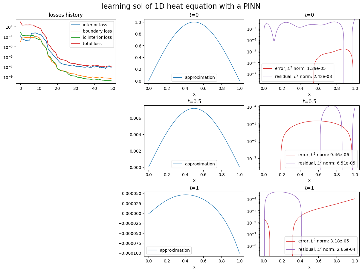
Approximation of the solution of a 1D heat equation

Let us now demonstrate how to define and train an PINN for a time dependent problem.

We consider the 1D heat equation

\[\partial_t u - \partial_{xx} u = 0 \text{ in } \Omega \times (0, T)\]

with boundary condition:

\[\partial_x u = g \text{ on } \partial \Omega \times (0, T)\]

and initial condition:

\[u = u_0 \text{ on } \Omega \times {0}\]

where \(u: \Omega \times (0, T) \to \mathbb{R}\) is the unknown function, \(\Omega \subset \mathbb{R}\) and \((0, T) \subset \mathbb{R}\). Neumann boundary conditions are prescribed, and the initial condition is a sinusoide.

Time and space domains

from scimba_jax.domains.meshless_domains.domains_1d import Segment1D

domain_t = (0.0, 1.0)
domain_x = Segment1D((0.0, 1.0), is_main_domain=True)

Sampler on \(\Omega\times T\)

from scimba_jax.nonlinear_approximation.integration.monte_carlo_time import (
    UniformTimeSampler,
)

sampler = TensorizedSampler(
    [
        UniformTimeSampler(domain_t),
        DomainSampler(domain_x),
    ],
    model_type="t_x",
    bc=True,
    ic=True,
)

Notice the optional arguments:

• model_type to specify the name and order of variables,

• bc to specify that samples are required for boundary condition,

• ic to specify that samples are required for initial condition.

Right-hand sides, initial and exact solution

Next we define the initial and the exact solutions. Again, notice the mu in the arguments of the function.

def exact_sol(t: jnp.ndarray, x: jnp.ndarray):
    return jnp.exp(-(t * jnp.pi**2)) * jnp.sin(jnp.pi * x)


def f_init(x: jnp.ndarray):
    t = jnp.zeros_like(x)
    return exact_sol(t, x)

Physical model

The model corresponding to the considered problem is already defined in scimba_jax.

from scimba_jax.physical_models.temporal_pde.heat_equations import HeatND

model = HeatND(
    main_domain=domain_x,
    time_domain=domain_t,
    bc="weak",
    ic="weak",
    f_ic_rhs=lambda *args: f_init(*args),
)

Other possible optional arguments are f_rhs and f_bc_rhs which are zero functions by default:

model = HeatND(
    main_domain=domain_x,
    time_domain=domain_t,
    bc="weak",
    ic="weak",
    f_rhs=lambda *args: jnp.zeros_like(args[0]),
    f_bc_rhs=lambda *args: jnp.zeros_like(args[0]),
    f_ic_rhs=f_init,
)

Approximation space

We wish to approximate the solution with a Multi-Layer Perceptron with 2 inputs (\(x\) and \(t\)), 1 output (\(u(t, x)\)) and two intermediate layers of \(16\) neurons each:

key = jax.random.PRNGKey(0)
nn = MLP(in_size=2, out_size=1, hidden_sizes=[16, 16], key=key)

space = ApproximationSpace(
    {"x": 1}, # here t is implicitly of dimension 1
    [(nn, "scalar", None)],
    model_type="t_x",
)

PINN training

We finally create a PINN with custom weights:

custom_weights = {"interior": [1.0], "boundary": [40.0], "ic interior": [100.0]}

pinn = Projector(model, space, sampler, weights=custom_weights)

N_COLLOC = 900
N_BC_COLLOC = 2000
N_IC_COLLOC = 2000
N_EPOCHS = 50

start = timeit.default_timer()
key, pinn = pinn.project(
    key, space, N_EPOCHS, N_COLLOC, N_BC_COLLOC, N_IC_COLLOC
)
end = timeit.default_timer()

plot_abstract_approx_space(
    pinn.space,
    domain_x,
    time_domain=domain_t,
    time_values=[0.0, 0.5, 1.0],
    loss=pinn.losses,
    residual=pinn.model,
    error=exact_sol,
    title="learning sol of 1D heat equation with a PINN",
)

Training: 100%|||||||||||||||||||| 50/50[00:22<00:00] , loss: 1.9e+01 -> 8.9e-08