Strong boundary conditions

In this second tutorial, we will see how to approximate the solutions of the problems of the previous tutorials using PINNs with strong boundary conditions.

Approximation of the solution of a parametric 2D Laplacian

We consider the equation:

\[- \mu \Delta u = 2(\mu\pi)^2 \sin(\pi x) \sin(\pi y)\]

on \((x,y) \in \Omega := [-1, 1]\times[-1, 1]\) with parameter \(\mu\in \mathbb{M}=[1,2]\) subject to the Dirichlet condition:

\[u = 0\]

on \(\partial\Omega\).

Let us first define some global variables then the right-hand side and the analytic solution.

N_COLLOC = 1000 # the number of collocation points for the interior residual
N_BC_COLLOC = 1000 # the number of collocation points for the boundary residual
N_EPOCHS = 50 # the number of steps of optimization
S_LAYERS = [16, 16] # the hidden layers widths of the MLPs defined below

import jax
import jax.numpy as jnp

def f_rhs(xy: jnp.ndarray, mu: jnp.ndarray) -> jnp.ndarray:
    x, y = xy[..., 0:1], xy[..., 1:2]
    return 2 * (mu[...,0:1] * jnp.pi)**2 * jnp.sin(jnp.pi * x) * jnp.sin(jnp.pi * y)

def analytic_solution(xy: jnp.ndarray, mu: jnp.ndarray) -> jnp.ndarray:
    x, y = xy[..., 0:1], xy[..., 1:2]
    return mu * jnp.sin(jnp.pi * x) * jnp.sin(jnp.pi * y)

Import all the modules we will need:

import timeit

from scimba_jax.domains.meshless_domains.domains_2d import Square2D
from scimba_jax.nonlinear_approximation.integration.monte_carlo import (
    DomainSampler,
    TensorizedSampler,
)
from scimba_jax.nonlinear_approximation.integration.monte_carlo_parameters import (
    UniformParametricSampler,
)
from scimba_jax.physical_models.elliptic_pde.laplacians import ParametricLaplacianDirichletND
from scimba_jax.nonlinear_approximation.networks.mlp import MLP
from scimba_jax.nonlinear_approximation.approximation_spaces.approximation_spaces import (
    ApproximationSpace,
)
from scimba_jax.nonlinear_approximation.numerical_solvers.projectors import Projector

Let us now define a PINN using strong boundary conditions.

First define the domains and the sampler; notice the bc=False as argument to the sampler.

domain_x = Square2D([(-1.0, 1.0), (-1.0, 1.0)], is_main_domain=True)

domain_mu = [(1., 2.)]
sampler = TensorizedSampler(
    [DomainSampler(domain_x), UniformParametricSampler(domain_mu)], bc=False
)

Use argument bc="strong" when defining the physical model:

model = ParametricLaplacianDirichletND(domain_x, f_rhs, bc="strong")

To enforce strongly the boundary conditions, we apply a post-processing the evaluation of the PINN:

def post_processing(
    approx: jnp.ndarray, xy: jnp.ndarray, mu: jnp.ndarray
) -> jnp.ndarray:
    x, y = xy[0:1], xy[1:2]
    return approx * (x + 1.0) * (1.0 - x) * (y + 1.0) * (1.0 - y)

Generate the approximation space using this post-processing:

key = jax.random.PRNGKey(0) #initialize the random generator
nn = MLP(in_size=3, out_size=1, hidden_sizes=S_LAYERS, key=key)
space = ApproximationSpace(
    {"x": 2, "mu": 1},       # x has dim 2, mu has dim 1
    [(nn, "scalar", None)],  # nn2 models a scalar function u
    model_type="x_mu",       # u depends of x and mu
    post_processing=post_processing # equip the space with the post-processing
)

Finally, define the PINN and train it as previously:

pinn = Projector(model, space, sampler)

start = timeit.default_timer()
key, pinn = pinn.project(key, space, N_EPOCHS, N_COLLOC)
end = timeit.default_timer()

print("time for %d epochs: " % N_EPOCHS, end - start)

print("interior loss after training: ", pinn.best_loss["interior"])
print("total    loss after training: ", pinn.best_loss["total"])

Training: 100%|||||||||||||||||||| 50/50[00:01<00:00] , loss: 5.9e+02 -> 3.6e-05
time for 50 epochs:  1.4012096249498427
interior loss after training:  [3.57481074e-05]
total    loss after training:  3.5748107424307674e-05

For the reference, let us define and train a PINN with weak boundary conditions (as in the previous tutorial):

sampler = TensorizedSampler(
    [DomainSampler(domain_x), UniformParametricSampler(domain_mu)], bc=True
)

model = ParametricLaplacianDirichletND(domain_x, f_rhs, bc="weak")

key = jax.random.PRNGKey(0) #initialize the random generator
nn2 = MLP(in_size=3, out_size=1, hidden_sizes=S_LAYERS, key=key)
space2 = ApproximationSpace(
    {"x": 2, "mu": 1},       # x has dim 2, mu has dim 1
    [(nn2, "scalar", None)],  # nn2 models a scalar function u
    model_type="x_mu",       # u depends of x and mu
)

pinn2 = Projector(model, space2, sampler)

start = timeit.default_timer()
key, pinn2 = pinn2.project(key, space2, N_EPOCHS, N_COLLOC)
end = timeit.default_timer()

print("time for %d epochs: " % N_EPOCHS, end - start)
print("interior loss after training: ", pinn2.best_loss["interior"])
print("boundary loss after training: ", pinn2.best_loss["boundary"])
print("total    loss after training: ", pinn2.best_loss["total"])

Training: 100%|||||||||||||||||||| 50/50[00:01<00:00] , loss: 1.1e+03 -> 1.3e-01
time for 50 epochs:  1.2606477921362966
interior loss after training:  [0.05734841]
boundary loss after training:  [0.007059]
total    loss after training:  0.12793839618710973

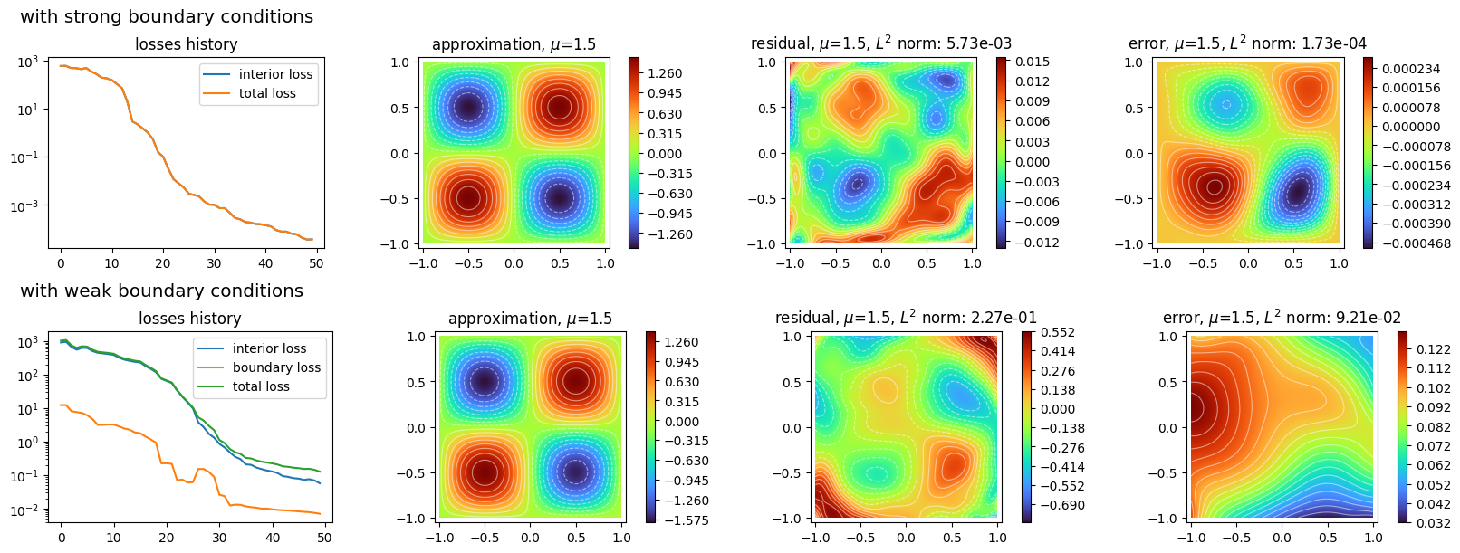
Plot the two PINNs:

import matplotlib.pyplot as plt
from scimba_jax.plots.plots_nd import plot_abstract_approx_spaces

plot_abstract_approx_spaces(
    (pinn.space, pinn2.space),  # the approximation spaces
    domain_x,  # the spatial domain
    domain_mu,  # the parameter's domain
    loss=(pinn.losses, pinn2.losses),  # for plot of the loss: the losses
    residual=(pinn.model, pinn2.model),  # for plot of the residual: the pde
    error=analytic_solution,  # for plot of the error with respect to a func: the func
    draw_contours=True,
    n_drawn_contours=20,
    titles=("with strong boundary conditions", "with weak boundary conditions"),
)
plt.show()

Approximation of the solution of a 1D heat equation

Let us now demonstrate how to define and train an PINN for a time dependent problem.

We consider the 1D heat equation

\[\partial_t u - \partial_{xx} u = 0 \text{ in } \Omega \times (0, T)\]

with boundary condition:

\[\partial_x u = g \text{ on } \partial \Omega \times (0, T)\]

and initial condition:

\[u = u_0 \text{ on } \Omega \times {0}\]

where \(u: \Omega \times (0, T) \to \mathbb{R}\) is the unknown function, \(\Omega \subset \mathbb{R}\) and \((0, T) \subset \mathbb{R}\). Neumann boundary conditions are prescribed, and the initial condition is a sinusoide.

We will demonstrate how to approximate the solution of this problem with three approaches:

• strong boundary condition and weak initial condition enforcement,

• weak boundary condition and strong initial condition enforcement,

• strong boundary condition and strong initial condition enforcement.

We define the initial condition:

def exact_sol(t: jnp.ndarray, x: jnp.ndarray):
    return jnp.exp(-(t * jnp.pi**2)) * jnp.sin(jnp.pi * x)


def f_init(x: jnp.ndarray):
    t = jnp.zeros_like(x)
    return exact_sol(t, x)

define global variables and import additional modules:

N_COLLOC = 900
N_BC_COLLOC = 2000
N_IC_COLLOC = 2000
N_EPOCHS = 50
S_LAYERS = [16, 16]

from scimba_jax.domains.meshless_domains.domains_1d import Segment1D
from scimba_jax.nonlinear_approximation.integration.monte_carlo_time import (
    UniformTimeSampler,
)
from scimba_jax.physical_models.temporal_pde.heat_equations import HeatND

We define the domains and the sampler. Here the sampler is common to the three approaches therefore it will always generate samples for the boundary and initial conditions, which is un-necessary but fine.

domain_t = (0.0, 1.0)
domain_x = Segment1D((0.0, 1.0), is_main_domain=True)

sampler = TensorizedSampler(
    [
        UniformTimeSampler(domain_t),
        DomainSampler(domain_x),
    ],
    model_type="t_x",
    bc=True,
    ic=True,
)

We define now the three post-processing functions corresponding to the three approaches we demonstrate below:

def post_processing_weak_ic_strong_bc(
    approx: jnp.ndarray, t: jnp.ndarray, x: jnp.ndarray
) -> jnp.ndarray:
    return approx * x * (1.0 - x)

def post_processing_strong_ic_weak_bc(
    approx: jnp.ndarray, t: jnp.ndarray, x: jnp.ndarray
) -> jnp.ndarray:
    return f_init(x) + approx * t

def post_processing_strong_ic_strong_bc(
    approx: jnp.ndarray, t: jnp.ndarray, x: jnp.ndarray
) -> jnp.ndarray:
    return f_init(x) + approx * t * x * (1.0 - x)

Defining and training a PINN with strong boundary condition and weak initial condition

model = HeatND(
    main_domain=domain_x,
    time_domain=domain_t,
    bc="strong",
    ic="weak",
    f_ic_rhs=lambda *args: f_init(*args),
)

key = jax.random.PRNGKey(0)
nn1 = MLP(in_size=2, out_size=1, hidden_sizes=S_LAYERS, key=key)

space1 = ApproximationSpace(
    {"x": 1},
    [(nn1, "scalar", None)],
    model_type="t_x",
    post_processing=post_processing_weak_ic_strong_bc
)

pinn1 = Projector(model, space1, sampler)

start = timeit.default_timer()
key, pinn1 = pinn1.project(
    key, space1, N_EPOCHS, N_COLLOC, n_ic_colloc=N_IC_COLLOC
)
end = timeit.default_timer()

Training: 100%|||||||||||||||||||| 50/50[00:01<00:00] , loss: 5.1e+00 -> 7.4e-08

Defining and training a PINN with weak boundary condition and strong initial condition

model = HeatND(
    main_domain=domain_x,
    time_domain=domain_t,
    bc="weak",
    ic="strong",
    f_ic_rhs=lambda *args: f_init(*args),
)

key = jax.random.PRNGKey(0)
nn2 = MLP(in_size=2, out_size=1, hidden_sizes=S_LAYERS, key=key)

space2 = ApproximationSpace(
    {"x": 1},
    [(nn2, "scalar", None)],
    model_type="t_x",
    post_processing=post_processing_strong_ic_weak_bc
)

pinn2 = Projector(model, space2, sampler)

start = timeit.default_timer()
key, pinn2 = pinn2.project(
    key, space2, N_EPOCHS, N_COLLOC, n_bc_colloc=N_BC_COLLOC
)
end = timeit.default_timer()

Training: 100%|||||||||||||||||||| 50/50[00:01<00:00] , loss: 3.7e+01 -> 1.1e-07

Defining and training a PINN with strong boundary condition and strong initial condition

model = HeatND(
    main_domain=domain_x,
    time_domain=domain_t,
    bc="strong",
    ic="strong",
    f_ic_rhs=lambda *args: f_init(*args),
)

key = jax.random.PRNGKey(0)
nn3 = MLP(in_size=2, out_size=1, hidden_sizes=S_LAYERS, key=key)

space3 = ApproximationSpace(
    {"x": 1},
    [(nn3, "scalar", None)],
    model_type="t_x",
    post_processing=post_processing_strong_ic_strong_bc
)

pinn3 = Projector(model, space3, sampler)

start = timeit.default_timer()
key, pinn3 = pinn3.project(
    key, space3, N_EPOCHS, N_COLLOC
)
end = timeit.default_timer()

Training: 100%|||||||||||||||||||| 50/50[00:01<00:00] , loss: 4.2e+01 -> 1.7e-07

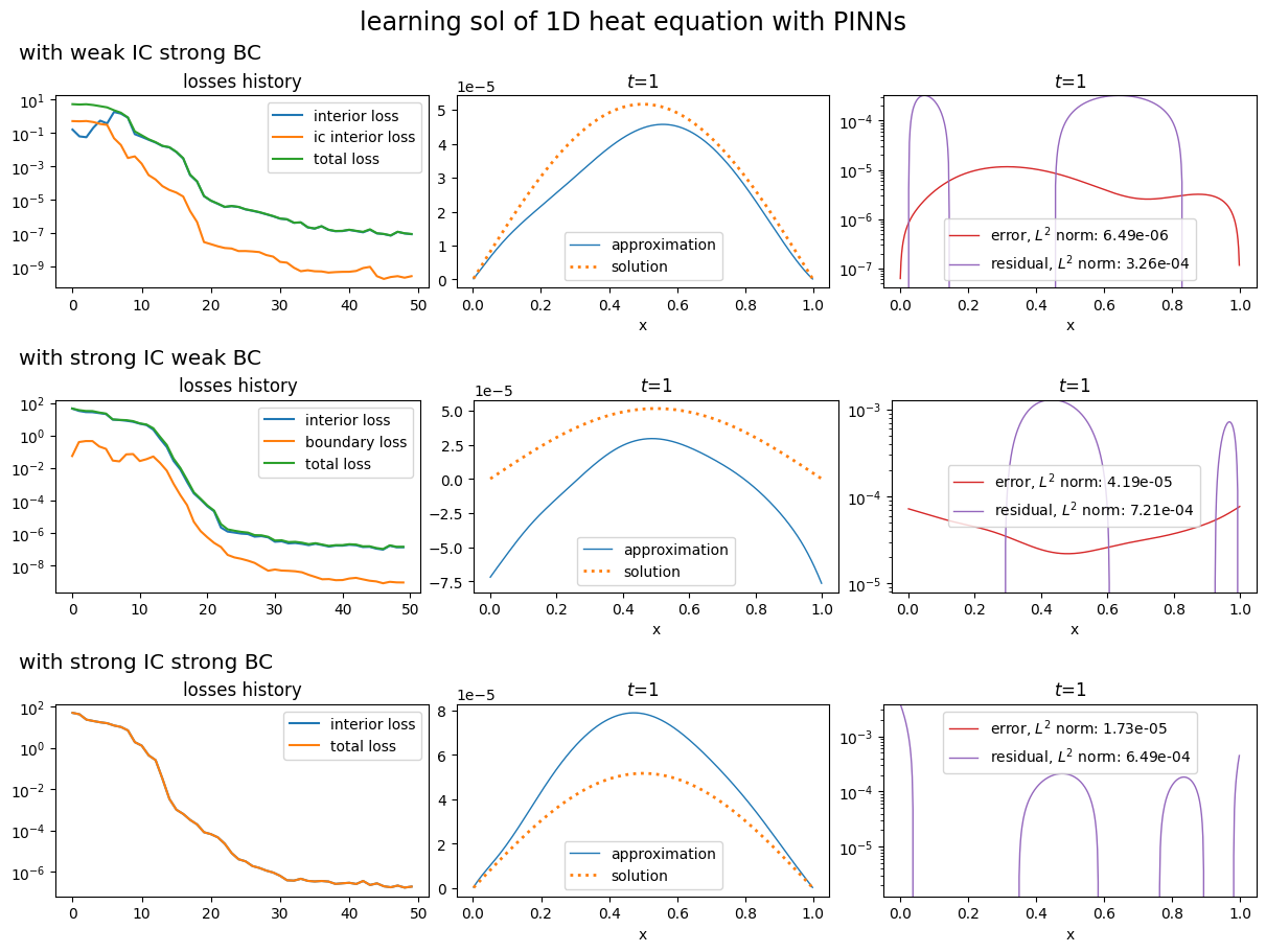
Compare the results

plot_abstract_approx_spaces(
    (pinn1.space, pinn2.space, pinn3.space),
    domain_x,
    time_domains=domain_t,
    loss=(pinn1.losses, pinn2.losses, pinn3.losses),
    residual=(pinn1.model, pinn2.model, pinn3.model),
    solution=exact_sol,
    error=exact_sol,
    title="learning sol of 1D heat equation with PINNs",
    titles=("with weak IC strong BC", "with strong IC weak BC", "with strong IC strong BC"),
)

plt.show()